Stott Expansion (resp. Contraction)
Within Verhandlingen der koninklijke Akademie van Wetenschappen, eerste Sectie, Deel XI (Amsterdam, published 1913 – but submitted already 1910)
Mrs. A. Boole Stott published the "Geometrical deduction of semiregular from regular polytopes and space fillings".
What is outlined there essentially boils down, by using Dynkin symbols, how polytopes are related which differ just in the mark of
a single node, i.e. changing an un-ringed node into a ringed one (or vice versa). – (For sure, this retrospective description
kind of is unfair, as her article well contributed to the understanding of these relations, and what now is known as Dynkin symbols
could be invented only thereafter in 1947 by Dynkin originally for Lie groups resp. 1948 by Coxeter as adoption to polytopes.)
If applied onto convex shapes only one might consider the polytope being contained within the rubber skin of a balloon. Then pulling apart
the vertices, all members of an edge class, those of a face class, or of any other bounding elements would just result in new edges (and
higher dimensional elements too) which simultanuously increase from zero to non-zero size (expansion). The inverse process, reducing
one specific edge class in size down to zero is called contraction.
A corresponding continuous transition can interactively be done in this VRML.
Despite of those few provided examples, Stott expansion applies to all dimensions and all curvatures, i.e.
spherical geometries as well as euclideans or
hyperbolics.
It should be pointed out that Stott expansion even commutes with alternated faceting (snubbing),
provided that snub nodes (s) and ringed nodes (x) are not directly connected by a link with mark n/d ≠ 2.
E.g. s4o3x could be derived from x4o3x
which is the Stott expansion of x4o3o by . . x (edges of o4o3x).
But likewise s4o3x is the Stott expansion of s4o3o by these edges, where
s4o3o itself was derived in turn from x4o3o. (Note that under this restriction each pair of the former ringed nodes
defines a square subelement, that is, the respective edges thus are always orthogonal.)
– Esp. in higher dimensions this observation proves quite useful to show whether an all unit edge variant for some
derived alternated faceting might exist: Whenever such a Stott contraction thereof was already shown to exist, then this holds
true for the symbol under consideration! E.g. s3s4o3o is known to exist as uniform figure,
therefore s3s4o3x would exist as unit-edge variant
(and thus as scaliform one) too.
Esp. with respect to the following section it should be pointed out, that full Stott expansion may be considered w.r.t. individual directions.
But any such direction then implies that simultanuous expansions will have to be applied in any further direction as well, which is an image
of the chosen one under the orbit of the refered to symmetry. –
Note that this original idea of Mrs. Stott applies not only to Coxeter groups only, i.e. to reflection derived groups which thus can be given by
Dynkin diagrams. This applies to any other symmetry as well. (Esp. as Mrs. Stott derived her ideas already years before the set up of Dynkin diagrams!)
This full Stott expansion (wrt. symmetry) was already called partial in some of her provided examples, e.g. when deriving the
tic out of the co. This was due to her missing possibility to take advantage of the
Dynkin symbols. So she was forced to just refer to the "limits" (nowadays we would say (sub-)facets) just by their dimension.
And when applying not to regular polytopes, but rather to Archimedean polytopes this already asks for different types of sub-facets of the specified dimension:
Even under full symmetry co obviously has 2 types of faces, squares and triangles. Still, even in these cases expansion
(or contraction) would always apply radially in normal direction.
Partial Stott Expansion (resp. Contraction)
To guarantee "semiregularity" (as she states it – nowadays we would ask for uniformity), the
application was meant to be restricted to actions under the full symmetry of the to be considered polytopes,
resp. to those symmetries which the unmarked Dynkin symbols represent themselves.
In the followings we will outline several types of more general applications.
In fact, we will distinguish in the followings 3 different levels of partiality.
(These will be outlined in more details below.)
-
partiality of 1st degree
-
just a single (to be specified) class (transiency under full symmetry!) of (sub-)facets (out of severals) defines the operation.
The operation always acts radially from some center. (For euclidean tesselations, this center also would be at infinity, for sure; like considering
those as polytopes in one dimension up having infinite radius.)
–
This usage already was mentioned by Mrs. Stott herself in her original paper.
-
partiality of 2nd degree
-
one or more (to be specified) classes (transiency under full symmetry!) of (sub-)facets defines the operation.
The operation acts on such sub-groups, and (for D-1 facets) needs no longer be directed along the facet normals.
(The latter would be necessary here, when it is just one class, for sure.)
–
This type of partiality was stressed a lot in the research for CRFs, esp. in 2014.
-
partiality of 3rd degree
-
either of the former would be applied wrt. some true subsymmetry only.
–
This is how the topic of (symmetry based) partial Stott expansions originally came up exactly 100 years after her publication
in distinct researches of Klitzing.
Partial Stott Expansion (resp. Contraction) of 2nd Degree
The seed examples here are expansions found in 2014 in a joint research for CRFs. They were based on
(different) facetings of the ike. Note how always patches of green facets (pentagons) and dark blue ones (triangles)
would move together – and thus "define" the corresponding action. This clearly exceed Mrs. Stott's original intend,
where no patches occured. Further in all cases the movements would be orthogonal to the axial direction,
and thus no longer along the face normals (which for patches not even would be defined any longer).
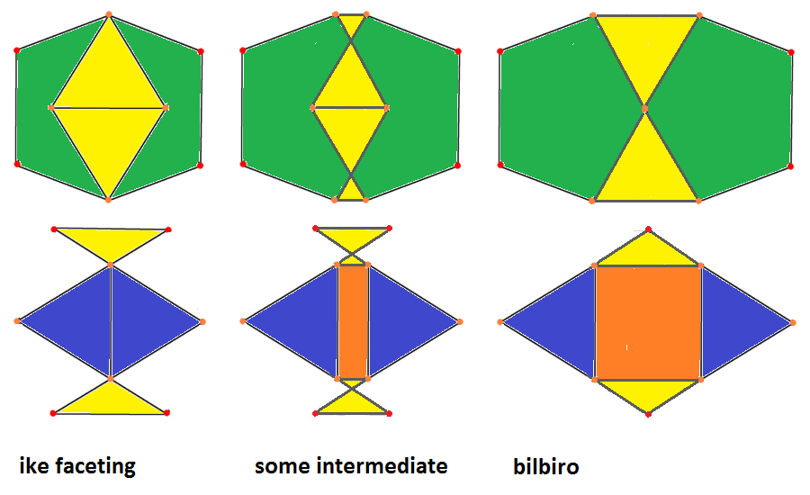
|
(-x)ofo(-x)-2-ofxfo &#xt

→ : (+x)-2-(+o) resp.
← : (-x)-2-(-o)

oxFxo-2-ofxfo &#xt (bilbiro, J91)
|
|
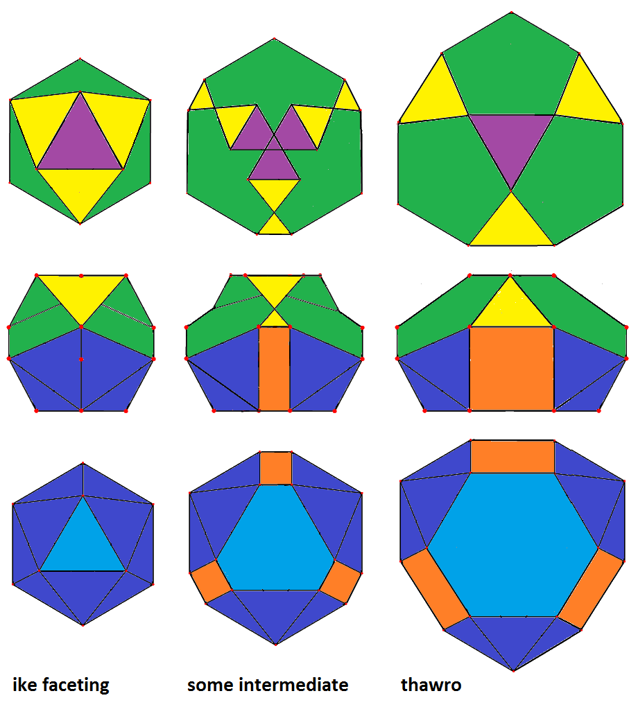
(-x)ofo-3-xfox &#xt

→ : (+x)-3-(+o) resp.
← : (-x)-3-(-o)

oxFx-3-xfox &#xt (thawro, J92)
|
|
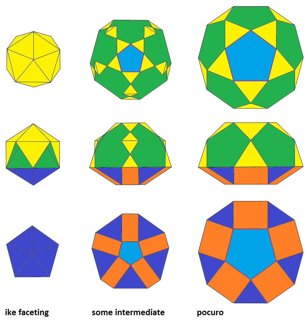
o(-x)oo-5-ofxo &#xt

→ : (+x)-5-(+o) resp.
← : (-x)-5-(-o)

xoxx-5-ofxo &#xt (pocuro, J32)
|
A similar process can be applied to other starting figures as well, even within other dimensions.
The most direct 4D examples became the axial applications of the formers to the icosahedral pyramid
which thus lead then to the find as well as the proof of existance of the 3 now so called pseudo-pyramids:
line || bilbiro,
{3} || thawro, and
{5} || pocuro – none of which is a segmentochoron by the way,
because of the lack of orbiformity.
But this research of those now so-called Expanded Kaleido-Facetings tracks a bit aside from the
clear view onto the mere topic of partial expansions (which there then will be used for one of their constructional steps only)
and thus deserves a separate page.
Partial Stott Expansion (resp. Contraction) of 3rd Degree
Exactly 100 years after the publication of Mrs. Stott's original paper, i.e. in 2013, Klitzing extended her ideas onto
sets of bounding elements, which form a complete equivalence class under some subsymmetry only. –
In general this would result in non-uniform polytopes.
(To be fair, it should be mentioned, that Mrs. Stott herself already mentioned rare subsymmetrical applications as an aside
on one page by her own. All these cases however where based between the relations of (hyper)cubic and demi(hyper)cubic polytopes,
where she obviously knew about the relation of elemental counts. Thence she used operators like
1/2c0 (contraction of half of the vertices) or
1/2e2 (expansion of half of the [triangular] faces).
But there is no clue onto more general subsymmetries, other than this quite exceptional occurance of "1/2".)
The main concern however was to result in CRF (convex regular faced) polytopes at least.
This restriction still was found to work at least within the following general setup:
Theorem
-
Let S1 be any pre-fix Dynkin subsymbol which is a linear sequence from o3 and x3 (possibly empty).
-
Let S2 be any post-fix Dynkin subsymbol which is a linear sequence from 3o and 3x (possibly empty).
-
Then there will be a partial Stott expansion series, starting at S1-o-2P-o-S2 and trailing
up to S1-o-2P-x-S2,
where 2P is some even positive integer.
-
Also there will be a partial Stott expansion series, starting at o-4-S1-o-4-o and trailing
up to o-4-S1-o-4-x.
-
Also there will be a partial Stott expansion series, starting at x-4-S1-o-4-o and trailing
up to x-4-S1-o-4-x.
-
Also there will be a partial Stott expansion series, starting at o-4-o-S2-4-o and trailing
up to o-4-x-S2-4-o.
-
Also there will be a partial Stott expansion series, starting at o-4-o-S2-4-x and trailing
up to o-4-x-S2-4-x.
-
Let |S1| be further the number of -3- links of that subsequence (possibly 0).
-
Then the number of transition steps of any such series can be given uniformly as: |S1| + 2.
For example, the picture below displays the case S1 = x3 and S2 being empty,
2P = 4:
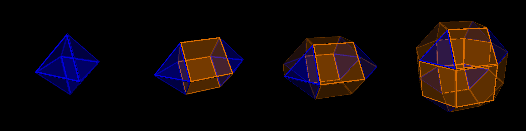
((qoo2oqo2ooq))&#zx  ↔ ((qoo2oqo2xxw))&#zx ↔ ((qoo2xwx2xxw))&#zx  ↔ ((wxx2xwx2xxw))&#zx
= x3o4o (oct)          (esquidpy)            (squobcu)              = x3o4x (sirco)
where: x = 1, q = sqrt(2), w = 1+sqrt(2)
Or the picture series below displays the case S1 = x3 and S2 being empty,
2P = 6:
hoo3oho3ooh3*a           ↔ hoo3oho3xxH3*a           ↔ hoo3xHx3xxH3*a              ↔ Hxx3xHx3xxH3*a
= x3o6o (trat)             (pextrat)                  (pacrothat)                   = x3o6x (rothat)
where: x = 1, h = sqrt(3), H = 1+sqrt(3)
In the followings the corresponding proof will be provided by explicit examples for the simpler ones (of any case),
grouped according to dimensions resp. space types: Any such family of series does contain at least a few series with uniform ones only.
There a classical Stott expansion series would apply – with respect to some subsymmetry (being explicitly given in the
corresponding footnote). From those subsymmetrical classical transitions it becomes clear, that the corresponding series
then even would be valid for the whole family in general as well. Moreover it becomes obvious, that similar families of series would
exist for the not explicitly provided higher dimensional cases too.
Some further examples beyond the scope of this theorem are known already, cf. below, esp. in the section on hyperbolic manifolds, or in the introduction of generalized hyperbolic tilings.
It should be mentioned however, that these subsequent transition steps of any such series not all fall into this partiality of 3rd degree.
Just each first transitions (in either direction) would break a higher symmetry. Thereafter it is broken already.
(Those following ones then would belong to the 2nd degree at most.)
-
Spherical Geometry: 2D – 3D – 4D – 5D
-
Euclidean Geometry: 2D – 3D – 4D
-
Hyperbolic Geometry: 2D – 3D
In the followings we use the subsequent idntifications for the various classes
|
†
|
subdimensional
|
|
°
|
uniform
|
|
*
|
scaliform
|
|
underline
|
Johnson solid / CRF
|
|
italic
|
CnRF = convex non-regular faced, i.e. showing up (still all-unit-edged) 2D-faces with various corner-angles
|
Spherical Geometry (up)
----
 2D
----
axial subsymmetry
o4o = point †°  ↔  edge †°   ↔  o4x = {4} °[1]

                                  o   o

  o              o   o            o   o
resulting in non-regular polygons:
x4o = {4} °     ↔  pexs      ↔  x4x = {8} °
                                   o   o
  o             o   o            o       o
o   o         o       o
  o             o   o            o       o
                                   o   o
triangular subsymmetry
o6o = point †°  ↔  {3} °     ↔  o6x = {6} °[2]
                                    o
                   o             o     o
  o             o
                   o             o     o
                                    o
----
 3D
----
prisms on 2D axial subsymmetry
x o4o = line †° ↔ {4} †° ↔ x o4x = cube °
resulting in non-regular polygons:
x x4o = cube ° ↔ pacop ↔ x x4x = op °
prisms on 2D triangular subsymmetry
x o6o = line †° ↔ trip ° ↔ x o6x = hip °
axial subsymmetry
o3o4o = point †° ↔ edge †° ↔ {4} †° ↔ o3o4x = cube °[3]
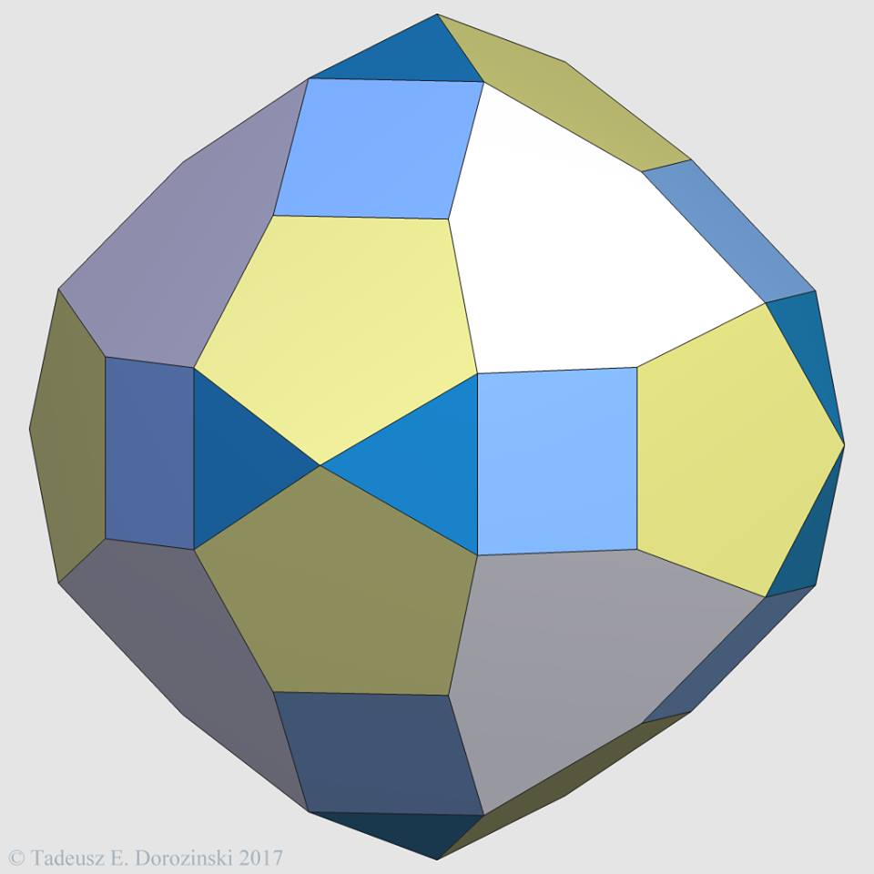
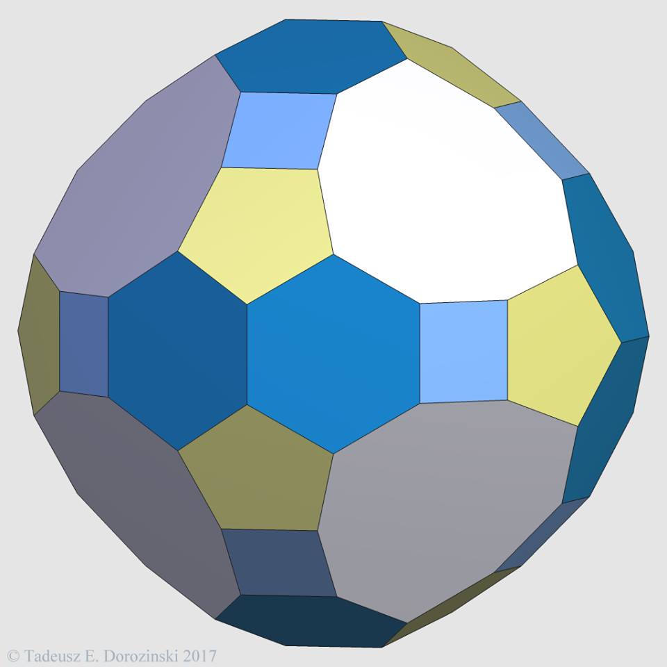
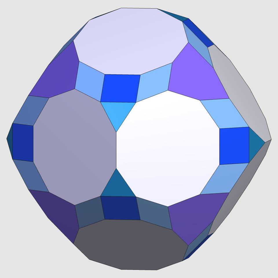
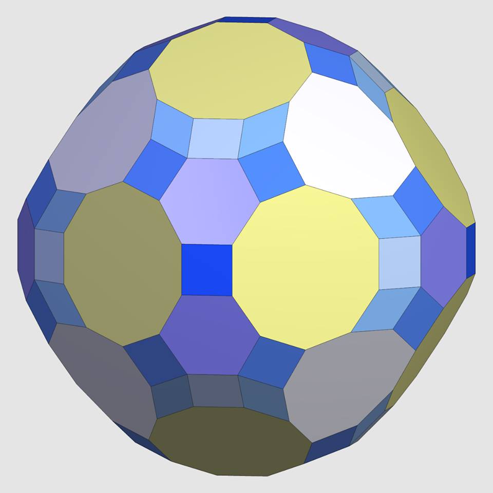
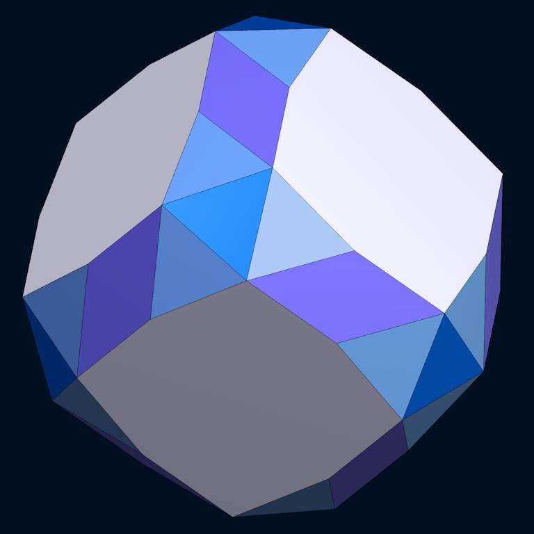
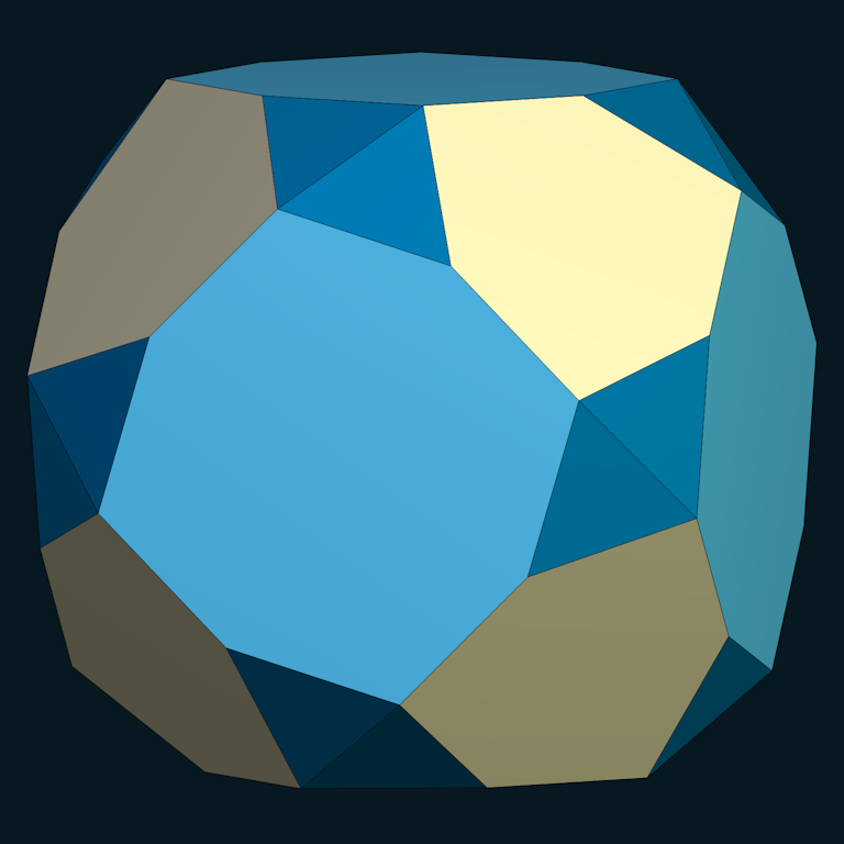
x3o4o = oct ° ↔ esquidpy ↔ squobcu ↔ x3o4x = sirco °[4]
It might be mentioned as an aside that those two sequences could be generalized, though not in the sense of 3 independent applications each,
but at least along a 1D direction (↔), resp. according to the symmetry of its 2D co-space (⇕).
resulting in non-regular polygons:
o3x4o = co °      ↔  pexco     ↔  pactic     ↔  o3x4x = tic °

x3x4o = toe °     ↔  pextoe    ↔  pac girco  ↔  x3x4x = girco °


o3o4s = tet °     ↔  pextet    ↔  pabextet   ↔  patex cube

x3o4s = tut °     ↔  pextut    ↔  pabextut   ↔  patex sirco
tetrahedral subsymmetry
o4o3o = point †°  ↔  tet °        ↔  o4x3o = co °[5]

o4o3x = oct °     ↔  tut °        ↔  o4x3x = toe °[6]
   | o4o3a    patex-o4o3a  o4x3a  :: tetrahedral
---+----------------------------
its 1st type of faces     (in the right case ever, in the left only for a = x):
 4 | . o3a    . o3a     -> . x3a  :: triangular
 4 | . o3a -> . x3a        . x3a
---+----------------------------
its 2nd type of faces     (in fact never):
12 | o . a    o . a        o . a  :: none
---+----------------------------
its 3rd type of faces     (in the right case ever, in the left one never):
 6 | o4o . -> pex-o4o   -> o4x .  :: axial
resulting in non-regular polygons:
x4o3o = cube °    ↔  patex cube   ↔  x4x3o = tic °

x4o3x = sirco °   ↔  patex sirco  ↔  x4x3x = girco °
octahedral subsymmetry
resulting in non-regular polygons:

 ©
o3o5x = doe ° ↔ phexdo x3o5o = ike ° ↔ phexik
  ©

o3o5x = doe °  ↔  phexdo      x3o5o = ike °  ↔  phexik
 ©
o3x5o = id ° ↔ phexid x3x5o = ti ° ↔ phexti o3x5x = tid ° ↔ phextid x3x5x = grid ° ↔ phexgrid
    ©

o3x5o = id °  ↔  phexid       x3x5o = ti °  ↔  phexti       o3x5x = tid °  ↔  phextid     x3x5x = grid °  ↔  phexgrid
 ©
 ©    ©

s3s4s = snic °  ↔  pox snic       s3s4s = snic °  ↔  padex snic
©
s3s4s = snic ° ↔ pox snic s3s4s = snic ° ↔ padex snic
square-pyramidal subsymmetry
resulting in non-regular polygons:
squippy ↔ pexsquippy (= pocsquacu) ↔ squacu
----
 4D
----
prismatic cases
x x3o4o = ope ° ↔ esquidpyp ↔ squobcupe ↔ x x3o4x = sircope °
pseudo-pyramids on 3D axial subsymmetry
ox3oo4oo&#x = octpy ↔ esquippidpy ↔ squicuf ↔ ox3oo4xx&#x = cubasirco
axial subsymmetry
o3o3o4o = point †°  ↔  edge †°   ↔  {4} †°          ↔  cube †°      ↔  o3o3o4x = tes °[7]

x3o3o4o = hex °     ↔  pex hex   ↔  quawros         ↔  pacsid pith  ↔  x3o3o4x = sidpith °[8]

o3x3o4o = ico °     ↔  pexic     ↔  bicyte ausodip  ↔  pacsrit      ↔  o3x3o4x = srit °

x3x3o4o = thex °    ↔  pex thex  ↔  pabex thex      ↔  pacprit      ↔  x3x3o4x = prit °
resulting in non-regular polygons:
o3o3x4o = rit °     ↔  pexrit    ↔  pabexrit        ↔  pactat       ↔  o3o3x4x = tat °

x3o3x4o = rico °    ↔  pexrico   ↔  pabexrico       ↔  pacproh      ↔  x3o3x4x = proh °

o3x3x4o = tah °     ↔  pextah    ↔  pabextah        ↔  pac grit     ↔  o3x3x4x = grit °

x3x3x4o = tico °    ↔  pextico   ↔  pabextico       ↔  pac gidpith  ↔  x3x3x4x = gidpith °
hexadecachoral or demitesseractic subsymmetry
o3o4o3o = point †°      ↔  hex °      ↔  rit °        ↔  o3o4x3o = rico °[9]

o3o4o3x = ico °         ↔  thex °     ↔  tah °        ↔  o3o4x3x = tico °[10]

x3o4o3o = (dual) ico °  ↔  poxic      ↔  pocsric      ↔  x3o4x3o = srico °

x3o4o3x = spic °        ↔  owau prit  ↔  poc prico    ↔  x3o4x3x = prico °
   | a3o4o3b    pox-a3o4o3b    poc-a3o4x3b    a3o4x3b  :: hexadecachoral
---+-------------------------------------------------
its 1st type of cells     (in the right case ever, in the left only for b = x):
 8 | . o4o3b -> . o4o3b        patex-o4o3b    . o4x3b  :: tetrahedral
 8 | . o4o3b    patex-o4o3b -> patex-o4o3b    . o4x3b
 8 | . o4o3b    patex-o4o3b    . o4x3b     -> . o4x3b
---+-------------------------------------------------
its 2nd type of cells     (in the right case for any b and a = x, in the left only for a = b = x):
32 | a . o3b    a . o3b        a . o3b     -> a . x3b  :: triangular
32 | a . o3b    a . o3b     -> a . x3b        a . x3b
32 | a . o3b -> a . x3b        a . x3b        a . x3b
---+-------------------------------------------------
its 3rd type of cells     (only for a = b = x):
96 | a3o . b    a3o . b        a3o . b        a3o . b  :: none
---+-------------------------------------------------
its 4th type of cells     (in the right case ever, in the left only for a = x):
24 | a3o4o . -> pex-a3o4o   -> pac-a3o4x   -> a3o4x .  :: axial
o4o3o3o = point †°  ↔  hex °   ↔  o4x3o3o = rit °[11]

o4o3x3o = ico °     ↔  thex °  ↔  o4x3x3o = tah °[12]

o4o3o3x = hex °     ↔  rit °   ↔  o4x3o3x = rico °[13]

o4o3x3x = thex °    ↔  tah °   ↔  o4x3x3x = tico °[14]
Note that the demitesseract is nothing but the hexadecachoron.
This is why this latter set of series already was contained by the former. (Cf. esp. the corresponding footnotes.)
resulting in non-regular polygons:
o3x4o3o = rico °        ↔  pox rico   ↔  poccont      ↔  o3x4x3o = cont °

o3x4o3x = srico °       ↔  pox srico  ↔  pibox srico  ↔  o3x4x3x = grico °

x3x4o3o = tico °        ↔  pox tico   ↔  pibox tico   ↔  x3x4x3o = (ico-dual) grico °

x3x4o3x = prico °       ↔  pox prico  ↔  poc gippic   ↔  x3x4x3x = gippic °
(A more consistent naming like "poc grico" wouldn't be unique here, as grico occurs in either of the ico-dual orientations. This is why the "pibox" adjective,
i.e. a "partially bi-octachorally expansion" is used here instead.)
o3o3o4x = tes °      ↔  pahtex tes      ↔  o3o3x4x = tat °

o3x3o4x = srit °     ↔  pahtex srit     ↔  o3x3x4x = grit °

x3o3o4x = sidpith °  ↔  pahtex sidpith  ↔  x3o3x4x = proh °

x3x3o4x = prit °     ↔  pahtex prit     ↔  x3x3x4x = gidpith °
icositetrachoric subsymmetry
((fox|o-3-ooo|f-3-xfo|o *b3-oxf|o))&#zx = ex ° ↔ ((fox|o-3-xxx|F-3-xfo|o *b3-oxf|o))&#zx = icau prissi
----
 5D
----
axial subsymmetry
o3o3o3o4o = point †°  ↔  edge †°  ↔  {4} †°     ↔  cube †°       ↔  tes †°     ↔  o3o3o3o4x = pent °[15]

x3o3o3o4o = tac °     ↔  pex tac  ↔  pabex tac  ↔  pabac scant   ↔  pac scant  ↔  x3o3o3o4x = scant °

o3x3o3o4o = rat °     ↔  pex rat  ↔  pabex rat  ↔  pabac span    ↔  pac span   ↔  o3x3o3o4x = span °

o3o3x3o4o = nit °     ↔  pexnit   ↔  pabexnit   ↔  pabac sirn    ↔  pacsirn    ↔  o3o3x3o4x = sirn °

x3x3o3o4o = tot °     ↔  pextot   ↔  pabextot   ↔  pabacca pin   ↔  pacca pin  ↔  x3x3o3o4x = cappin °

x3o3x3o4o = sart °    ↔  pex sart ↔  pabex sart ↔  pabac carnit  ↔  paccarnit  ↔  x3o3x3o4x = carnit °

o3x3x3o4o = bittit °  ↔  ...      ↔  ...        ↔  ...           ↔  ...        ↔  o3x3x3o4x = prin °

x3x3x3o4o = gart °    ↔  ...      ↔  ...        ↔  ...           ↔  ...        ↔  x3x3x3o4x = cogart °
demipenteractic subsymmetry
o4o3o3o3o = point †°  ↔  hin °     ↔  o4x3o3o3o = rin °[16]

o4o3x3o3o = nit °     ↔  thin °    ↔  o4x3x3o3o = bittin °[17]

o4o3o3x3o = rat °     ↔  sirhin °  ↔  o4x3o3x3o = sibrant °[18]

o4o3x3x3o = bittit °  ↔  girhin °  ↔  o4x3x3x3o = gibrant °[19]

o4o3o3o3x = tac °     ↔  siphin °  ↔  o4x3o3o3x = spat °[20]

o4o3x3o3x = sart °    ↔  pithin °  ↔  o4x3x3o3x = pirt °[21]

o4o3o3x3x = tot °     ↔  pirhin °  ↔  o4x3o3x3x = pattit °[22]

o4o3x3x3x = gart °    ↔  giphin °  ↔  o4x3x3x3x = gippit °[23]
duoprismatic subsymmetry
o3o3o3o3o = hix ° ↔ pexhix ↔ pabex hix *[24]
----
 2D  = tilings
----
axial subsymmetry
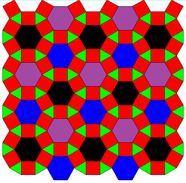
o4o4o = point †°  ↔  aze †°   ↔  o4o4x = squat °[25]

x4o4o = squat °   ↔  squat °  ↔  x4o4x = squat °[26]
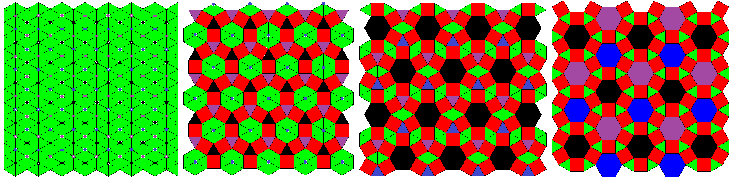
The transitions of the second series might be described like this: all red squares (left) ↔ alternating "columns" of red and blue squares (center)
↔ alternating both the columns (red / blue) and the rows (say: red / yellow), thereby providing additional green squares at the
crossings of blue columns and yellow rows (right). –
Note that an even higher order transition would be implied by the idea provided further below for general xNo4x.
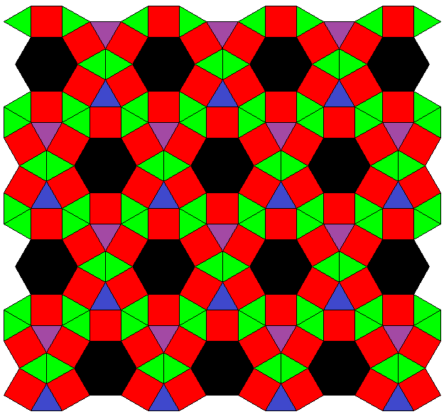
o4o4o = point †°  ↔  aze †°     ↔  o4x4o = squat °[25]

o4o4x = squat °   ↔  tosquat °  ↔  o4x4x = tosquat °
The transitions of the second series might be described like this: alternating yellow and red squares, vertices marked blue (left) ↔
yellow octagons, red squares again, and the pairwise octagon connections marked blue (center) ↔
again yellow octagons, red octagons plus blue squares (right).
– Thus those 2 latter tosquats would be relatively aligned with a 45 ° rotation!
tri-pesic subsymmetry
o3o6o = point †°           ↔  trat °                    ↔  that °                    ↔  o3o6x = hexat °[27]

x3o6o = trat °             ↔  pextrat                   ↔  pacrothat                 ↔  x3o6x = rothat °
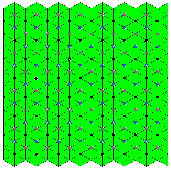
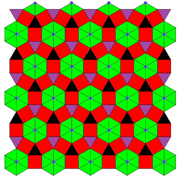
Note that this family so far is not covered by the theorem above. But the same technique applies here too. Even the number of transition steps could be calculated by the same formula.
The transitions of the second series, which is also depicted above, might be described like this: 3-coloring of vertices into e.g. black, purple, blue, while all triangles are alike, e.g. green (outer left) ↔
only the former black-purple edges expand to squares, former black and purple verices become additional triangles, green triangles remain as before (center left) ↔
former black-blue edges expand to squares, black triangles become hexagons, blue vertices become triangles, green and purple triangles remain as before (center right) ↔
former purple-blue edges finally expand into squares too, purple and blue triangles become hexagons too, green triangles still remain as before (outer right).
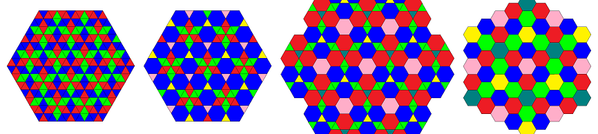
((xAoo3xoAo3xooA3*a))&#zx ↔ ((uBxx3xoAo3xooA3*a))&#zx ↔ ((uBxx3uxBx3xooA3*a))&#zx ↔ ((uBxx3uxBx3uxxB3*a))&#zx °
This partial Stott sequence (with A=3x, B=4x=2u) was found in 2014 by
Gevaert
with analogue means, as where used some months before within the CRF research,
which then lead to the figures provided under partiality of 2nd degree.
The existance of rhombs in the first three sequence members makes this one non-CRF so.
----
 3D  = honeycombs
----
axial subsymmetry
o4o3o4o = point †°  ↔  aze †°   ↔  squat †°  ↔  o4o3o4x = chon °[28]

x4o3o4o = chon °    ↔  chon °   ↔  chon °    ↔  x4o3o4x = chon °[29]

o4x3o4o = rich °    ↔  pexrich  ↔  pacsrich  ↔  o4x3o4x = srich °

x4x3o4o = tich °    ↔  pextich  ↔  pacprich  ↔  x4x3o4x = prich °
o3o3x *b4o = octet ° ↔ pextoh * ↔ pacratoh * ↔ o3o3x *b4x = ratoh °
The last series could be considered as an alternating faceting of the second series of the former block:
we have s4o3o4y = o3o3x *b4y (where y=o or y=x). Similarily one might ask about the further alternated faceting case.
But that one does not provide anything new, within this symmetry it just reproduces the 3rd sequence: s4x3o4y = o4x3o4y.
alternated-cubic-honeycombal subsymmetry
o4o3o4o = point †°  ↔  octet °   ↔  o4x3o4o = rich °[30]

o4o3x4o = rich °    ↔  tatoh °   ↔  o4x3x4o = batch °[31]

o4o3o4x = chon °    ↔  ratoh °   ↔  o4x3o4x = srich °[32]

o4o3x4x = tich °    ↔  gratoh °  ↔  o4x3x4x = grich °[33]
----
 4D  = tetracombs
----
axial subsymmetry
o4o3o3o4o = point †°   ↔  aze †°   ↔  squat †°  ↔  chon †°  ↔  o4o3o3o4x = test °[34]

x4o3o3o4o = test °     ↔  test °   ↔  test °    ↔  test °   ↔  x4o3o3o4x = test °[35]

o4x3o3o4o = rittit °   ↔  ...      ↔  ...       ↔  ...      ↔  o4x3o3o4x = sidpitit °

o4o3x3o4o = icot °     ↔  ...      ↔  ...       ↔  ...      ↔  o4o3x3o4x = srittit °

x4x3o3o4o = tattit °   ↔  ...      ↔  ...       ↔  ...      ↔  x4x3o3o4x = capotat °

x4o3x3o4o = srittit °  ↔  ...      ↔  ...       ↔  ...      ↔  x4o3x3o4x = scartit °

x4x3x3o4o = grittit °  ↔  ...      ↔  ...       ↔  ...      ↔  x4x3x3o4x = gicartit °
hexadecachoric-tetracombal subsymmetry
o3o3o4o3o = point †°   ↔  hext °   ↔  rittit °   ↔  bricot °  ↔  o3o3o4x3o = ricot °[36]

o3o3o4o3x = icot °     ↔  thext °  ↔  batitit °  ↔  bithit °  ↔  o3o3o4x3x = ticot °[37]

x3o3o4o3o = hext °     ↔  ...      ↔  ...        ↔  ...       ↔  x3o3o4x3o = spaht °

x3o3o4o3x = scicot °   ↔  ...      ↔  ...        ↔  ...       ↔  x3o3o4x3x = capoht °

o3x3o4o3o = icot °     ↔  ...      ↔  ...        ↔  ...       ↔  o3x3o4x3o = sibricot °

o3x3o4o3x = spict °    ↔  ...      ↔  ...        ↔  ...       ↔  o3x3o4x3x = paticot °

x3x3o4o3o = thext °    ↔  ...      ↔  ...        ↔  ...       ↔  x3x3o4x3o = pataht °

x3x3o4o3x = capicot °  ↔  ...      ↔  ...        ↔  ...       ↔  x3x3o4x3x = capticot °
    | a3b3o4o3c    phextex-a3b3o4o3c  pabhextex-a3b3o4o3c  phextco-a3b3o4x3c  a3b3o4x3c  :: hexadecachoric-tetracombal
----+----------------------------------------------------------------------------------
its 1st type of cells     (in the right case ever, in the left only for b = x or c = x):
  N | . b3o4o3c -> . b3o4o3c          pox-b3o4o3c          poc-b3o4x3c        . b3o4x3c  :: hexadecachoral
  N | . b3o4o3c    pox-b3o4o3c     -> pox-b3o4o3c          poc-b3o4x3c        . b3o4x3c
  N | . b3o4o3c    pox-b3o4o3c        poc-b3o4x3c       -> poc-b3o4x3c        . b3o4x3c
  N | . b3o4o3c    pox-b3o4o3c        poc-b3o4x3c          . b3o4x3c       -> . b3o4x3c
----+----------------------------------------------------------------------------------
its 2nd type of cells     (in the right case only for a = x, in the left only for a = c = x):
 8N | a . o4o3c    a . o4o3c          a . o4o3c         -> patex-o4o3a-p   -> a . o4x3c  :: tetrahedral
 8N | a . o4o3c    a . o4o3c       -> patex-o4o3a-p        patex-o4o3a-p      a . o4x3c
 8N | a . o4o3c    a . o4o3c          patex-o4o3a-p        patex-o4o3a-p      a . o4x3c
 8N | a . o4o3c -> patex-o4o3a-p      patex-o4o3a-p     -> a . o4x3c          a . o4x3c
 8N | a . o4o3c    patex-o4o3a-p      patex-o4o3a-p        a . o4x3c          a . o4x3c
 8N | a . o4o3c    patex-o4o3a-p   -> a . o4x3c            a . o4x3c          a . o4x3c
----+----------------------------------------------------------------------------------
its 3rd type of cells     (in the right case only for a = x or b = x, in the left only for (a = x or b = x) and c = x):
32N | a3b . o3c    a3b . o3c          a3b . o3c            a3b . o3c       -> a3b . x3c  :: triangular
32N | a3b . o3c    a3b . o3c          a3b . o3c         -> a3b . x3c          a3b . x3c
32N | a3b . o3c    a3b . o3c       -> a3b . x3c            a3b . x3c          a3b . x3c
32N | a3b . o3c -> a3b . x3c          a3b . x3c            a3b . x3c          a3b . x3c
----+----------------------------------------------------------------------------------
its 4th type of cells     (only for (a = x or b = x) and c = x):
96N | a3b3o . c    a3b3o . c          a3b3o . c            a3b3o . c          a3b3o . c  :: none
----+----------------------------------------------------------------------------------
its 5th type of cells     (in the right case ever, in the left only for a = x or b = x):
12N | a3b3o4o . -> pex-a3b3o4o     -> pabex-a3b3o4o     -> pac-a3b3o4x     -> a3b3o4x .  :: axial
(dual) hexadecachoric-tetracombal subsymmetry
o3o4o3o3o = point †°   ↔  hext °     ↔  rittit °   ↔  o3o4x3o3o = bricot °[38]

o3o4o3x3o = icot °     ↔  thext °    ↔  batitit °  ↔  o3o4x3x3o = bithit °[39]

o3o4o3o3x = hext °     ↔  rittit °   ↔  bricot °   ↔  o3o4x3o3x = ricot °[40]

o3o4o3x3x = thext °    ↔  batitit °  ↔  bithit °   ↔  o3o4x3x3x = ticot °[41]

x3o4o3o3o = icot °     ↔  ...        ↔  ...        ↔  x3o4x3o3o = sricot °

x3o4o3x3o = spict °    ↔  ...        ↔  ...        ↔  x3o4x3x3o = pricot °

x3o4o3o3x = scicot °   ↔  ...        ↔  ...        ↔  x3o4x3o3x = scaricot °

x3o4o3x3x = capicot °  ↔  ...        ↔  ...        ↔  x3o4x3x3x = gicaricot °
Note that the first 4 of these series each are subseries of the first 2 series of the former block, cf. the corresponding footnotes.
alternated-tesseractic-tetracombal subsymmetry
o4o3o3o4o = point †°   ↔  hext °      ↔  o4x3o3o4o = rittit °[42]

o4o3x3o4o = icot °     ↔  thext °     ↔  o4x3x3o4o = batitit °[43]

o4o3o3x4o = rittit °   ↔  bricot °    ↔  o4x3o3x4o = ricot °[44]

o4o3x3x4o = batitit °  ↔  bithit °    ↔  o4x3x3x4o = ticot °[45]

o4o3o3o4x = test °     ↔  siphatit °  ↔  o4x3o3o4x = sidpitit °[46]

o4o3x3o4x = srittit °  ↔  pithatit °  ↔  o4x3x3o4x = prittit °[47]

o4o3o3x4x = tattit °   ↔  pirhatit °  ↔  o4x3o3x4x = potatit °[48]

o4o3x3x4x = grittit °  ↔  giphatit °  ↔  o4x3x3x4x = gippittit °[49]
In contexts of hyperbolical uniform tilings (of any dimensions) one generally is used to embed the infinite polytopal incidence structure right
into the supporting manifold itself. For euclidean space this would be natural, and for spherical geometry this would be an alternate,
so not often used display for uniform convex polytopes: their projection from the body center onto the vertex (hyper-)sphere.
For hyperbolically infinite non-uniform polytopes on the other hand this might not be the best way of display any longer.
This is because the supporting manifold surely should contain at least the vertices, and then would no longer be defined uniquely:
There might be cases with varying curvature too, and then the vertex separation would allow for different,
i.e. analytic versus non-analytically continuous changes thereof.
Having said this, we'd rather propagate the natural way of display for spherical geometries here as well: the embedding of the geometry
into an euclidean space of one dimension plus.
I.e. instead of considering a tesselation of a manifold one rather uses (here: infinite) polytopes.
Thereby then all used sub-polytopes too would live in according euclidean
subspaces in turn: all edges remain straight, all polygons remain flat, etc. And there will be that additional extrinsic measurement
derived from the embedding space: I.e. any regular triangle could thus be represented with their usual 60° corners,
even for all hyperbolc things under consideration!
In the context of partial Stott expansions this "scrumbled quilt" representation of hyperbolic non-uniform polytopes
is of special interest. This is because the expansion operation itself acts in a (locally) euclidean way.
E.g. the elongated square dipyramid kind of adds a cylindric part between the 2 hemispheres (when seen as tiling). That is, if we'd
stick to hyperbolic tiling display, we'd get regions which would not change the so far used curvature, while the squashed in expansion regions
then, although being completely connected to the formers, would use zero curvature. On the other hand, when using that euclidean embedding,
this neither does baffle in spherical nor would it for the partial expansion when being applied here to hyperbolic geometries.
(In the context of classical Stott expansion, this did not emerge so far: because the expansion application there uses the same
symmetry as the uniform starting figure itself, instead of a subsymmetry. This then surely results in a different figure, which will
always be uniform again and thus esp. has a single vertex class. Therefore it can be represented readily as tiling of a manifold of
constant curvature again, which will be defined by the new vertex set alone.)
----
 2D  (hyperbolic manifold)
----
o3o4o3*a = point †°  ↔  pex-o3o4o3*a °  ↔  pabex-o3o4o3*a °  ↔  pac-o3o4x3*a  ↔  o3o4x3*a °

x3o4o3*a °           ↔  pex-x3o4o3*a    ↔  pabex-x3o4o3*a    ↔  pac-x3o4x3*a  ↔  x3o4x3*a °
This small set of series exceeds the proposition of the introductory theorem in 2 ways:
Because the base symmetry symbol contains a loop, it clearly is not contained in the there stated preconditions.
But even the there followed line of proof would not apply either, as the simplest base series (the first one) here can not take refuge to
a classical Stott series, just because not all of its members qualify as uniform!
xNo4x allows for a consistent N-coloring of the squares in rhombi-symmetrical positions (i.e. the x . x squares), one for each side of the N-gons.
Accordingly any such square can be contracted into pairs of incident (and thus to be identified) edges independently. I.e. for any subset choice out of this set of N elements (up to equivalences)
there will be an according partial Stott contraction (resp. expansion, when starting at the corresponding N-coloring of edges of xNo4o).
N=3 here clearly would revolve back to 3D axials of spherical geometry.
Thereby stating nothing but what was given there.
Similarily N=4 would revolve back to 2D axials of euclidean geometry.
In this case showing, beyond the there given series, that parallel expansions might be alternated in turn!
– What differs between the there provided transition series and the one here brought up is that the final (colored) tiling
there was still uniform, but here clearly is not! (Speaking of colored objects, the final member in the corresponding N=3 case
then would not be uniform either.)
----
 3D  (hyperbolic manifold)
----
o3x3o3*a4o °  ↔  pex-o3x3o3*a4o *  ↔  pac-o3x3o3*a4x *  ↔  o3x3o3*a4x °

o3x3x3*a4o °  ↔  pex-o3x3x3*a4o    ↔  pac-o3x3x3*a4x    ↔  o3x3x3*a4x °
This family of series also exceeds the cited theorem because the prefixed Dynkin subsymbol contains a loop and so the precondition is not met.
(In fact, the calculation rule here too would come out wrong.)
Moreover this family kind of is exceptional furtheron, because a formaly corresponding series between o3o3o3*a4o (point) and
o3o3o3*a4x simply does not exist! – Just suppose the existance of an hypothetical
"pac-o3o3o3*a4x". That one would require 3 squares per edge already from any "ry"-square
layer of o3o3o3*a4x (cf. its 3-coloring of edges, contracting the "b"-edges),
and thus, overall (from any of the to be adjoined "parallel" layers), ∞-many squares at any edge.
Thus this would become an extremely non-dyadic square complex, rather than some hyperbolic polyhedron –
and hence has to be excluded from consideration.
o3o6o3o = point †°  ↔  pex-o3o6o3o °  ↔  pac-o3o6x3o °  ↔  o3o6x3o °[50]

o3o6o3x °           ↔  pex-o3o6o3x °  ↔  pac-o3o6x3x °  ↔  o3o6x3x °[51]

x3o6o3o °           ↔  ...            ↔  ...            ↔  x3o6x3o °

x3o6o3x °           ↔  ...            ↔  ...            ↔  x3o6x3x °
That paracompact honeycomb transition family already incorporates this euclidean tiling transition family with
tri-pesic subsymmetry (as contained horohedra). So too, this family so far is not covered by the theorem above.
But none the less its technique applies here still. Also the number of transition steps could be calculated by the same formula correctly.
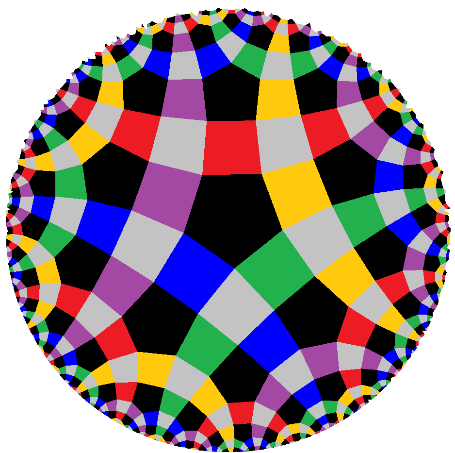
There is a consitent 12-coloring of the pentagons of x5o3o4o (one per face of each dodecahedron).
– In fact, the pentagons of x5o3o4o fall in subdimensional tilings of type x5o4o.
Those tilings intersect orthogonally.
Thus the above mentioned edge coloring of the latter induces that face coloring of the former. –
Therefore for any subset choice out of this set of 12 elements (up to equivalences) there will be an according partial Stott expansion,
introducing layers of pentagonal prisms, and possibly, if all 3 pairwise orthogonal sub-tilings at a
vertex of x5o3o4o are concerned, some cubes. –
Gradually this leads towards x5o3o4x.
(Respectively backwards from that one: there thus is a
consistent 12-coloring of its pentagonal prisms, which allows for corresponding partial Stott contractions.)
And, restricted to the just mentioned sub-tiling, that one would then gradually become x5o4x,
for sure.
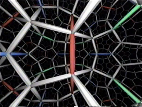
A similar partial Stott expansion by pentagonal prisms can be applied to the hypercompact hyperbolic honeycomb
x3o3o5o5*a, when shifting the former bollocells pepat slightly apart.
This then results in pex-x3o3o5o5*a, being found at the end of 2025.
Aside: Some of the above partial Stott sequences (with uniforms only) can be re-written as classical Stott sequences too,
just by using a lower symmetry right from the beginning:
- ↑:
o o ↔ x o ↔ x x
- ↑:
o3o ↔ x3o ↔ x3x
- ↑:
o o o ↔ x o o ↔ x x o ↔ x x x
- ↑:
((qoo oqo ooq))&#zx ↔ ((wxx oqo ooq))&#zx ↔ ((wxx xwx ooq))&#zx ↔ ((wxx xwx xxw))&#zx
- ↑:
o3o3o ↔ x3o3o ↔ x3o3x
- ↑:
o3x3o ↔ x3x3o ↔ x3x3x
- ↑:
o o o o ↔ x o o o ↔ x x o o ↔ x x x o ↔ x x x x
- ↑:
((qooo oqoo ooqo oooq))&#zx ↔ ((wxxx oqoo ooqo oooq))&#zx ↔ ((wxxx xwxx ooqo oooq))&#zx ↔ ((wxxx xwxx xxwx oooq))&#zx ↔ ((wxxx xwxx xxwx xxxw))&#zx
- ↑:
o3o3o *b3o ↔ x3o3o *b3o ↔ x3o3x *b3o ↔ x3o3x *b3x
- ↑:
o3x3o *b3o ↔ x3x3o *b3o ↔ x3x3x *b3o ↔ x3x3x *b3x
- ↑:
o3o3o *b3o ↔ x3o3o *b3o ↔ x3o3x *b3o
- ↑:
o3x3o *b3o ↔ x3x3o *b3o ↔ x3x3x *b3o
- ↑:
o3o3o *b3x ↔ x3o3o *b3x ↔ x3o3x *b3x
- ↑:
o3x3o *b3x ↔ x3x3o *b3x ↔ x3x3x *b3x
- ↑:
o o o o o ↔ x o o o o ↔ x x o o o ↔ x x x o o ↔ x x x x o ↔ x x x x x
- ↑:
o3o3o *b3o3o ↔ x3o3o *b3o3o ↔ x3o3x *b3o3o
- ↑:
o3x3o *b3o3o ↔ x3x3o *b3o3o ↔ x3x3x *b3o3o
- ↑:
o3o3o *b3x3o ↔ x3o3o *b3x3o ↔ x3o3x *b3x3o
- ↑:
o3x3o *b3x3o ↔ x3x3o *b3x3o ↔ x3x3x *b3x3o
- ↑:
o3o3o *b3o3x ↔ x3o3o *b3o3x ↔ x3o3x *b3o3x
- ↑:
o3x3o *b3o3x ↔ x3x3o *b3o3x ↔ x3x3x *b3o3x
- ↑:
o3o3o *b3x3x ↔ x3o3o *b3x3x ↔ x3o3x *b3x3x
- ↑:
o3x3o *b3x3x ↔ x3x3o *b3x3x ↔ x3x3x *b3x3x
- ↑:
oo3xo oo3ox&#x ↔ xx3xo oo3ox&#x ↔ xx3xo xx3ox&#x
- ↑:
((o∞o)) ((o∞o)) ↔ ((o∞o)) ((x∞o)) ↔ ((x∞o)) ((x∞o))
- ↑:
((x∞o)) ((x∞o)) ↔ ((x∞o)) ((x∞x)) ↔ ((x∞x)) ((x∞x))
- ↑:
o3o3o3*a ↔ x3o3o3*a ↔ x3x3o3*a ↔ x3x3x3*a
- ↑:
((o∞o)) ((o∞o)) ((o∞o)) ↔ ((o∞o)) ((o∞o)) ((x∞o)) ↔ ((o∞o)) ((x∞o)) ((x∞o)) ↔ ((x∞o)) ((x∞o)) ((x∞o))
- ↑:
((x∞o)) ((x∞o)) ((x∞o)) ↔ ((x∞o)) ((x∞o)) ((x∞x)) ↔ ((x∞o)) ((x∞x)) ((x∞x)) ↔ ((x∞x)) ((x∞x)) ((x∞x))
- ↑:
o3o3o *b4o ↔ x3o3o *b4o ↔ x3o3x *b4o
- ↑:
o3x3o *b4o ↔ x3x3o *b4o ↔ x3x3x *b4o
- ↑:
o3o3o *b4x ↔ x3o3o *b4x ↔ x3o3x *b4x
- ↑:
o3x3o *b4x ↔ x3x3o *b4x ↔ x3x3x *b4x
- ↑:
((o∞o)) ((o∞o)) ((o∞o)) ((o∞o)) ↔ ((o∞o)) ((o∞o)) ((o∞o)) ((x∞o)) ↔ ((o∞o)) ((o∞o)) ((x∞o)) ((x∞o)) ↔ ((o∞o)) ((x∞o)) ((x∞o)) ((x∞o)) ↔ ((x∞o)) ((x∞o)) ((x∞o)) ((x∞o))
- ↑:
((x∞o)) ((x∞o)) ((x∞o)) ((x∞o)) ↔ ((x∞o)) ((x∞o)) ((x∞o)) ((x∞x)) ↔ ((x∞o)) ((x∞o)) ((x∞x)) ((x∞x)) ↔ ((x∞o)) ((x∞x)) ((x∞x)) ((x∞x)) ↔ ((x∞x)) ((x∞x)) ((x∞x)) ((x∞x))
- ↑:
o3o3o *b3o *b3o ↔ x3o3o *b3o *b3o ↔ x3o3x *b3o *b3o ↔ x3o3x *b3x *b3o ↔ x3o3x *b3x *b3x
- ↑:
o3x3o *b3o *b3o ↔ x3x3o *b3o *b3o ↔ x3x3x *b3o *b3o ↔ x3x3x *b3x *b3o ↔ x3x3x *b3x *b3x
- ↑:
o3o3o *b3o *b3o ↔ x3o3o *b3o *b3o ↔ x3o3x *b3o *b3o ↔ x3o3x *b3x *b3o
- ↑:
o3x3o *b3o *b3o ↔ x3x3o *b3o *b3o ↔ x3x3x *b3o *b3o ↔ x3x3x *b3x *b3o
- ↑:
o3o3o *b3o *b3x ↔ x3o3o *b3o *b3x ↔ x3o3x *b3o *b3x ↔ x3o3x *b3x *b3o
- ↑:
o3x3o *b3o *b3x ↔ x3x3o *b3o *b3x ↔ x3x3x *b3o *b3x ↔ x3x3x *b3x *b3x
- ↑:
o3o3o *b3o4o ↔ x3o3o *b3o4o ↔ x3o3x *b3o4o
- ↑:
o3x3o *b3o4o ↔ x3x3o *b3o4o ↔ x3x3x *b3o4o
- ↑:
o3o3o *b3x4o ↔ x3o3o *b3x4o ↔ x3o3x *b3x4o
- ↑:
o3x3o *b3x4o ↔ x3x3o *b3x4o ↔ x3x3x *b3x4o
- ↑:
o3o3o *b3o4x ↔ x3o3o *b3o4x ↔ x3o3x *b3o4x
- ↑:
o3x3o *b3o4x ↔ x3x3o *b3o4x ↔ x3x3x *b3o4x
- ↑:
o3o3o *b3x4x ↔ x3o3o *b3x4x ↔ x3o3x *b3x4x
- ↑:
o3x3o *b3x4x ↔ x3x3o *b3x4x ↔ x3x3x *b3x4x
- ↑:
o3o3o3o3*a3*c *b3*d ↔ o3x3o3o3*a3*c *b3*d ↔ o3x3x3o3*a3*c *b3*d ↔ o3x3x3x3*a3*c *b3*d
- ↑:
x3o3o3o3*a3*c *b3*d ↔ x3x3o3o3*a3*c *b3*d ↔ x3x3x3o3*a3*c *b3*d ↔ x3x3x3x3*a3*c *b3*d
 ©
©