| Site Map | Polytopes | Dynkin Diagrams | Vertex Figures, etc. | Incidence Matrices | Index |
Take a small (hyper)sphere situated at a vertex, then the intersection of its surface with the polytope defines the vertex figure. Often this (hyper)spherical tesselation is represented by a corresponding polytope. Topological this figure is equivalent to the (sub-dimensional) dual of that facet of the dual polytope which corresponds to that chosen vertex (of the original polytope).
As the edges incident to the chosen vertex show up in the vertex figure as its vertices, the faces incident to the chosen vertex show up as its edges, etc. the numbers of that figure show up in the incidence matrix of the original polytope as the superdiagonal part of the matrix row which corresponds to the chosen vertex.
In a stricter sense for spherical space uniform polytopes, when embedded into euclidean space of one dimension above, one could consider an orientation of the polytope with one vertex taken as the top-most one. Then the vertex figure can be derived as the section of that polytope with an affine hyperplane, situated at the one but top-most vertex layer. - This in fact is nothing but the sefa (sectioning facet) underneath a vertex. And this too is what will be reffered to in the next section as the metrically correct vertex figure, when being derived by means of the Dynkin symbol.
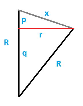
Using this metrically correct vertex figure, then there can be derived a nice formula, relating the circumradii of the original polytope (R) and of the vertex figure polytope (r): From the graphic at the right one easily derives (using the edge length x): r2 = x2 - p2. Similarily one has r2 = R2 - (R - p)2 = 2Rp - p2. Therefrom one freely gets x2 = 2Rp. Now solving for p and then inserting that into the first equation results in r2 = (4R2 - x2) x2 / 4R2. If we use unit edge lengths, then this relation even can be simplified to r2 = 1 - 1 / 4R2 or, what is equivalent, R2 = 1 / 4(1 - r2).
Note that for spherical cases R generally is real. – Accordingly (as 2R always is ≥ x = 1) r will be real, and 0 ≤ r < 1.
For euclidean cases R gets infinite. – Accordingly r will be = 1.
For hyperbolic cases R is purely imaginary. – Then r would get > 1.
In rare hyperbolic cases R is itself 0 i. – Then we get r being positive infinite.
For quasiregular polytopes the vertex figure is easily derived. Just omit the ringed node and the incident links. Ring instead the previously neighboring nodes. More precisely the edges, corresponding to those new ringed nodes, will have to be sized differently, each according to the vertex figure of the sub-diagram consisting out of the original node, the neighboring node under consideration, and the (now deleted) link in between.
How this works is shown for x3o4o (oct), in order to demonstrate that this concept also works for quasiperiodic polytopes independent of whether the links marked 2 are used or omitted in Dynkin diagrams. The direct application of the above said demand the vertex figure to be x(3)-4-o. Here the number in parentheses represents the mark of the omitted link. Quite generally the function x(.) results in (an edge of) the length of the first chord of the corresponding polygon, i. e. represents the vertex figure of that specific polygon. For instance the vertex figure of a triangle is just the opposite edge, thus x(3) = x. Therefore the above derived vertex figure just is x4o. More generally, these length values are given by
  x(2) : x  = 0
  x(3) : x  = 1
  x(4) : x  = 1.414214
  x(5) : x  = 1.618034
  x(6) : x  = 1.732051
  x(∞) : x  = 2
  x(p) : x  = sin(2π/p)/sin(π/p) for p>1
Some special cases Miss Krieger has given single characters just for abreviation (cf. also notation elements of Dynkin symbols). These are:
  x(3)   = x
  x(4)   = q
  x(5)   = f
  x(5/2) = v
  x(6)   = h
  x(∞)   = u
Note, the "full" diagram of the above used starting polytope (oct) would be x3o4o2*a, if no links would be sub-pressed. Its vertex figure thence would be accordingly x(3)-4-x(2). But the vertex figure of a dyad is just its opposite vertex, therefore the side corresponding to x(2) is degenerate, having zero length, cf. the above listing. Thus this edge could be neglected as well, and the incident vertices could be identified. Then we get again, just as already followed above from the reduced diagram, as vertex figure the square x4o.
As alternate example consider o3o3x4o (rit). Its vertex figure, in this metrically correct notation, will be given accordingly by the diagram o-3-x(3) . x(4). Thus it is essentially a triangular prism, but the base faces are scaled as having unit edges (vertex figure of triangle), contrasting to the lacing edges, which are of size sqrt(2) (vertex figure of square).
For polytopes with Dynkin diagrams, where more than just one node is ringed, things get a bit more complicate. This is where the concept of lace simplices needs to come in. This concept (up to my knowledge) is due to Miss Krieger.
First one splits the diagram into several sub-diagrams by deleting all but one ringed node each and omits further all links incident to the deleted nodes. The vertex figures of all those subgraphes (derived in the above sense, as those now represent quasiregulars only) are then to be used as the parallel layers of the lace simplex. Make sure to derive those metrically exact. These derived layers will be connected pairwise by lacings which in turn are exactly the vertex figures of the subgraphs consisting out of any 2 of the original ringed nodes (plus the connecting link, if existent).
As a first easy example, the vertex figure of x3x4o (toe) is derived. The layers would be verf(x . o) and verf(. x4o). The vertex figure of a dyad is just a point, that of the square a line of length sqrt(2). In this example we further have just one kind of lacings: verf(x3x .), i.e. a line of length sqrt(3). Thus we got a triangular vertex figure which is a point above a sqrt(2) base, laced by sqrt(3) sides (which in this trivial example could have been derived directly as the 3 vertex figures of the faces incident to each vertex).
Again giving a more complex alternate example. The vertex figure of o3x3x4x (grit) is derived by the layers verf(o3x . .), verf(o . x .), and verf(o . . x). Thus those layers are a unit length edge (vertex figure of the triangle) and 2 points (vertex figures of the dyads). These layers now are laced by verf(. x3x .), verf(. x . x), respectively verf(. . x4x) edges, that is the former unit edge is joined to the first point by sqrt(3) edges (vertex figure of hexagon), to the second point by sqrt(2) edges (vertex figure of square), and the 2 points are joined by an edge of length 2*sin(135°/2) ≈ 1.847759 (vertex figure of octagon).
Not totally different, but kind of an extreme case, is the consideration of the vertex figure of a cross product polytope. Consider for example the duoprism x3o x5o (trapedip). The layers are clearly verf(x3o . o) = . x(3) . . respectively verf(. o x5o) = . . . x(5), ie. edges of length 1 respectively tau. And the lacing edges here are verf(x . x .) only, ie. edges of length sqrt(2). What is more interesting, those top and bottom edges do not belong to the same 2-dimensional subspace, as can be seen from the given Dynkin diagrams, ie. the vertex figure becomes not a flat trapezium, they rather are to be placed orthogonally, so that the vertex figure becomes a kind of digonal antiprism. More generally any duoprism P x Q has as vertex figure a wedge with layers verf(P) respectively verf(Q), and those layers are placed within the mutually perpendicular subspaces of P respectively Q. Especially, the latteral facets are pyramides only, connecting facets of P to vertices of Q and vice versa.
Theory could be expanded even further. The vertex figures in turn of those latter rather special lace prisms with orthogonal arranged layers can be easily derived as well, as the used cells are either the top or bottom figure or pyramids. So they clearly are either verf(verf(P)) atop orthogonal verf(Q) or the other way round. And as edge figures are nothing but the vertex figures of vertex figures, and so on for even higher figures, the set of all those figures for quasiregular polytopes is easily derivable. Consider for example the diagram o3o3x3o3o3o (bril), if "&#x" is used to denote the lacing edges, respectively "||" is used to denote 'atop' (see here):
. . . . . . -figure of  o3o3x3o3o3o  is  o3x . x3o3o              =  o3x . . . . x . . . x3o3o

. . x . . . -figure of  o3o3x3o3o3o  is  xo .. .. .. ox3oo&#x(4)  =  x . . . . . || . . . . x3o

. o3x . . . -figure of  o3o3x3o3o3o  is  .. .. .. .. ox3oo&#x(4)  =  . . . . . . || . . . . x3o
. . x3o . . -figure of  o3o3x3o3o3o  is  xo .. .. .. .. ox&#x(4)  =  x . . . . . || . . . . . x

o3o3x . . . -figure of  o3o3x3o3o3o  is  .. .. .. .. .x3.o        =                . . . . x3o
. o3x3o . . -figure of  o3o3x3o3o3o  is  .. .. .. .. .. ox&#x(4)  =  . . . . . . || . . . . . x
. . x3o3o . -figure of  o3o3x3o3o3o  is  xo .. .. .. .. oo&#x(4)  =  x . . . . . || . . . . . .

o3o3x3o . . -figure of  o3o3x3o3o3o  is  .. .. .. .. .. .x        =                . . . . . x
. o3x3o3o . -figure of  o3o3x3o3o3o  is  .. .. .. .. .. ..&#x(4)  =  . . . . . . || . . . . . .
. . x3o3o3o -figure of  o3o3x3o3o3o  is  x. .. .. .. .. ..        =  x . . . . .
The sectioning facets underneath the to be alternated element of a snub is well worth to be considered separately. However, its deduction is quite analog to the formal derivation of the vertex figure above. In fact, just remember that for Coxeter snubs (i.e. having s and o nodes solely), the sefa is nothing but the verf of its starting figure. And thereby remember that the starting figure was obtained by simply replacing the s nodes by x nodes. When it now comes towards true Klitzing snubs (i.e. having not just s and o nodes only, but having additional x nodes too), then remember that those could be seen as a Stott expansion of an according Coxeter snub, i.e. the one where the x nodes got reduced to o nodes again. That is, keeping this in mind, then the former sefa derivation rule for Coxeter snubs too gets globally overlayed by that very Stott expansion process.
Thus putting the above together, it simply runs as follows:
Consider for example the (non-rescaled) sefa of prissi = s3s4o3x:
0.   s3s4o3x
1.   s3s4o3o
2.   x3x4o3o
3a.  verf( x / o3o ) = . / o3o
3b.  verf( / x4o3o ) = / . q3o
3c.  verf( x3x / / ) = h
3.   .. .. oq3oo&#h
4.   .. .. oq3xx&#h
(which, because rescaling back to all unit edges, in case to be allowed by according degrees of freedom, happens to be possible within that case, finally indeed results in nothing but tricu = ox3xx&#x).
For polyhedra the vertex figures become especially simple denotable, as the faces become represented by lines of different length, and exactly 2 such lines connect at those points, which are the cross-sections of the edges incident to the chosen vertex. That is those face-representing lines make up circuits (which well can have multiple windings, crossings, etc.). Thus vertex figures of polyhedra can be denoted by sequences of incident face types. Most often this looks like
[3,4,5,4]
for the small rhombicosidodecahedron (sirco). If sub-sequences are repeated, this can be denoted using a power notation, such as
[(3,4)2]
for the cuboctahedron (co). Further the winding number has to be considered. There are sequences that spool several times around the vertex. As winding numbers of faces are denoted by quotients, this notation is taken over to vertex figures as well. Thence
[35]/2
denotes the vertex figures of the great icosahedron (gike). On the other hand it might even wind to and fro with a total being null. Here we have to be a bit careful. Consider a crossed trapezoid where the parallel lines remain. Then the center with respect to the vertices is completely within one loop and the winding number nevertheless is 1. But if we consider a crossed trapezoid where the lacings remain that vertex center is completely outside the figure, and we have a total winding number of 0. For the intermediate case of a crossed rectangle, where the diagonal lines are incident to the center, both views could be applied as limiting cases, but as a divisor being 0 looks a bit strange, in those cases we favor the number 1. Thus we denote
[3/2,43] resp. [3/2,4,3,4] but [8/7,4/3,8,4]/0
for the vertex figures of the quasirhombicuboctahedron (querco), the octahemioctahedron (oho), respectively the small rhombihexahedron (sroh). And finally vertices might coincide (without necessarily making the solid figure itself to a compound). Here an additive notation is chosen. For instance the Grünbaum polyhedron which looks like an cubohemioctahedron plus 4 tetrahedrally arranged {6/2} (cho+4{6/2}) would have as vertex figure
2[6/2,4,6]
Truncation is a physical process applicable to any polytope, which is ment as cutting off some or all vertex pyramids more or less deepely. (Having spoken of vertex pyramids, it becomes clear that – for this very reason – truncation depth will be restricted such that this intersection (hyper)plane still intersects the vertex emanating edges. – In more specialised cases some deeper truncations will be considered below.) In the context of a vertex transitive symmetry, an according application to all vertices is understood. (Therefore alternatively it could be understood to be the intersection with an apropriately scaled dual polytope.) Moreover it is obvious that those cut-off pyramids then will have to be upright, i. e. the base would be orthogonal to the axis of symmetry. This base polytope of the pyramid further more will be the vertex figure of the polytope to be truncated. Note that independently of the depth of truncation the geometry of the additional facets introduced by truncation is fixed (up to size), at least as long as those from different positions do not intersect. In opposition to that, the length of the former edges clearly gets smaller and smaller, depending on the depth of truncation. The limiting case, where the intersections of the truncating hyperplanes of neighbouring vertices will just meet at the middle of the former edge, further is called rectification.
Although one is used to apply this operation most generally to highly symmetrical polytopes like regulars or quasiregulars (see below), it well can be applied too at other polytopes as well. In this generality however, it leaves the realm of uniform polytopes. Examples would be the truncation resp. the rectification of sadi, i.e. tisadi resp. risadi.
With respect to quasiregular polytopes, truncation in any depth (down till their next vertex intersection) can be given explicitly in the Dynkin diagramatical description with full metrical correctness. Consider here as an example the rectified hecatonicosachoron o3o3x5o (rahi). The vertex figure of which according to the above is o-3-x(3) . x(5). Here it follows what is derived:
  o-3--o--3--x--5--o  : starting polytope
  o-3-x(3)   .   x(5) : vertex figure
  o-3-x(3)-3-t-5-x(5) : truncated polytope
Here the relative depth of truncation is modelled by the size of the edge marked t. For t = 0 the former edges would be reduced to nothing, thereby representing the limiting case of the rectified polytope. While on the other hand for t = ∞ the length of the former edges would overcome any finite length by far, therefore representing the untruncated polytope again.
Note that allthough this t can be chosen independingly, and thus could be used to get the uniform representant (which has all edges of the same length), this will not be possible in this case here, because of the independant non-uniform geometry of the vertex figure itself. None the less there is a representant in the same topological equivalence class, even having all facet planes parallel to the true truncate, which is uniform. That one can be obtained by replacing both, all x(p) and t, by the unit edges x. Thus in the case of consideration that uniform representant of the truncate would be o3x3x5x (grahi). On the other hand, the uniform representant of the rectified version would be o3x3o5x (srahi). This btw. is the deeper sense because e.g. the great rhombicuboctahedron (girco) also is known as the "truncated cuboctahedron".
For regular polytopes even deeper "truncations" can be considered as well. Then the dual polytope, the one which is used for intersection, is regular as well, and can be given within the same symmetry group (i.e. its Dynkin diagram will have the same structure, only that the opposite end node is the one being ringed instead). This gives rise to a complete truncational series, best being described by an explicit example:
x3o3o5o  - regular base polytope (ex)
x3x3o5o  - truncation (tex)
o3x3o5o  - rectification (rox)
o3x3x5o  - bi-truncation (xhi)
o3o3x5o  - bi-rectification (rahi)
o3o3x5x  - tri-truncation (thi)
o3o3o5x  - (... and finally:) dual (hi)
Obviously one-ringed and two-adjoined-ringed states do alternate. In fact, the n-truncational states can be made also continuously filling the gaps between the n-rectates, just by applying different edge scales to those two-ringed states (i.e. applying 2 variables x and y instead), running from one-to-zero up to zero-to-one.
This sequence of different polytopes of that truncational series finally could further be understood as an sectioning series perpendicular to an additional dimension, i.e. of a polytope within one dimension higher. That very higher-dimensional polytope then technically would be an antitegum, i.e. the dual of that antiprism, which in turn is derived as the segmentotope "regular polytope || dual polytope".
 © ©
|
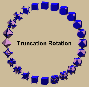
But there is a different extension of the truncational process as well. That different one moves the intersection points of the truncating (hyper-)plane along the arbitrarily extended edge-lines of the starting figure. The difference here is that both, beyond the starting figure (negative positions, outside of the starting polytope), as well as positive positions beyond the rectified polytope, would lead to non-convex shapes. Here the positions can be moved from -∞ to +∞. And, if additionally the overall size all the way through is scaled down to a given circumradius, then the finite size of the former figure would get down to zero in those limiting cases. Doing so would lead to the so called truncation rotation, i.e. a process which would close projectively those limiting points into one. That truncation parameter would be z = ±∞ at the left, would be z = 0 (i.e. no truncation at all) at the top, would be z = 1/2 at the right, and z = 1 (i.e. the intersection points reach the opposite end of the former edges) at the bottom in the diplay of the nearby shown picture. – In fact, the top-right realm from z = 0 to z = 1/2 clearly is the usual truncation, as already described above. The bottom-right realm from z = 1/2 to z = 1 is known as hypertruncation. The bottom-left one from z = 1 to z = +∞ is known as quasitruncation. Finally the remaining top-left realm of negative z-parameters is both known as inflected truncation and as antitruncation. In fact, when applied to the cube, as in the shown pictures, this could likewise be described by means of the Coxeter-Dynkin diagram o3y4x, where the edge size x is being kept unity throughout, while the parameter y is running between y = +∞ and y = -∞. Then the above truncation parameter would be given by z = y/(x+y). I.e. we have y = 0 at the top, y = 1 at the right, y = ±∞ at the bottom, and y = -1 at the left. – Sure, the pictures further got rescaled to a common height throughout. In the language of kaleidoscopical Wythoff construction this sequence is being described when spotting that edge of the fundamental simplex, which runs from the vertex to the edge midpoint of a regular polytope. If this edge would be extrapolated into the full supporting line instead and the defining seed point of the kaleidoscopical construction would be anywhere on that line, then any individual instance of this sequence would be derived again. |
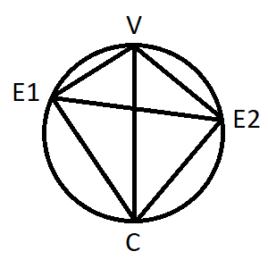
For general isogonal polytopes with different incident edge types however, the situation becomes a bit more arbitrary. Consider the diagram of an polygonal case to the right. V represents a vertex, C the center of the polygon. E1 and E2 represent the mid-points of the respective incident edges (sides). The edge-radii C-E1 resp. C-E2 clearly are orthogonal onto the edges, as represented by the also being shown circle of Thales.
The afore mentioned truncation hyperplane so far was assumed to be arranged dually in the sense of spherical reciprocation, i.e. orthogonal to the circumradius C-V. This is why we spoke above, dealing there with truncations in their stricter sense, of cutting off an upright vertex pyramid. But when having different incident edge types, esp. when those are of different size as shown in the picture, there would be no symmetry driven need to restrict a cutting hyperplane to be orthogonal only. And furthermore, when considering rectification resp. ambification below, where the considered truncation depth gets chosen such that the hyperplane shall intersect the edge mid-points each, would require (and thus allow for) non-orthogonal cuts as well, then for instance parallel to E1-E2 instead.
The etymology here is a bit dull. Sure, rectification stems from latin rectificare, i.e. getting s.th. right, but that says nothing about the corresponding geometrical process to be applied here. In the context of Wythoffian polytopes, it clearly is correlated to that specific quasiregular case, where the second node is ringed only (oPxQoRo...). As such it is closely related to the process of truncation. In fact, the truncation depth has to be chosen such, that the 2 intersection points of those hyperplanes wrt. to the end points (i.e. vertices) of any edge just coincide.
It should be noted that truncation as such not only is well-defined for Wythoffian polytopes, but more generally for any isogonal polytope. Then the truncation has to be applied in the same way to all vertices, and thus this understanding of rectification here is well-defined too. We note that in all these contextes the resulting point of coincidence happens to be the midpoint of the corresponding edge, right by virtue of assumed symmetry equivalence of both its ends.
Conway more recently introduced therefore a second operational term, ambo, when referring to construct a new polytope right from the midpoints of the edges of a former polytope. – The etymology of "ambo" derives from αμβων, i.e. is greek and means "elevate", e.g. like a pulpit. Thus it is not less obscure to its operational process, but still it implies some symmetry. – Such an operation then clearly can be applied to any starting polytope.
As soon as we would assume an action of some sub-symmetry or even genuinely multi-gonal polytopes, i.e. multiple vertex classes, then the truncation depth clearly needs only be the same at any of the vertex classes individually, but no longer throughout. Accrodingly a rectification then in general no longer is well-defined. And even if, then it no longer is forced to result in the former edge midpoints generally. Therefore the operation of rectify and ambo here no longer coincide anymore.
Examples of figures, where rectification indeed can be applied to multi-gonal polytopes, are the duals of the (Wythoffian) rectified polychora, i.e. to the Catalans oPmQoRo. It is immediate that quite generally any truncation (and thus a potential rectification too) of a polytope would result in an according truncation of its former cells. Therefore we can take our focus on these. Here the only cells are bipyramids oxoRooo&#yt = ((co oxRoo))&#zy (for lacing edges of some size y and some tip-to-tip distance c). Their equatorial edges use same vertices on both sides. Therefore there a corresponding rectification point is immediate. But then the according truncational hyperplanes also define further points on the lacing edges too. Because the tips on the other hand are isolated, a there being applied truncation can be accomodated accordingly to match all these points on the former lacing edges simultanuously. Obviously the such defined points then generally are different from the midpoints of the former lacing edges. (Just the single case o3m3o4o happens to be regular itself.)
The resulting rectified figures priviously had been described by Gévay as non-Wythoffian perfect polytopes. (Perfect polytopes by definition do not allow for variations without changing the action of its symmetry group on its face-lattice.) Within tegum sum notation they can then be given as ((oaPooQboRoc))&#zx, where a and b edges only qualify as pseudo edges wrt. the full polychora. Although Gévay constructed these polychora in a different way, his attribution of perfectness directly correlates to the current point of interest! For, whenever using different points on the lacing edges of those bipyrmaids instead, their rhombic truncational faces of their equatorial vertices would break up into pairs of triangles.
| Symmetry oPoQoRo | Catalan oPmQoRo = d ( oPxQoRo ) | Gévay polychoron r ( oPmQoRo ) |
|---|---|---|
| o3o3o3o | o3m3o3o = ((co3oo3oo3ox))&#zy | ((oq3oo3qo3oc))&#zx |
| o3o3o4o | o3m3o4o = ((qo3oo3oo4ox))&#zy = ico (regular) | ((oq3oo3qo4ox))&#zx = rico (Wythoffian) |
| o3o3o5o | o3m3o5o = ((co3oo3oo5ox))&#zy | ((oq3oo3qo5oc))&#zx |
| o3o4o3o | o3m4o3o = ((co3oo4oo3ox))&#zy | ((oa3oo4bo3oc))&#zx |
| o4o3o3o | o4m3o3o = ((co4oo3oo3ox))&#zy | ((oa4oo3bo3oc))&#zx |
| o5o3o3o | o5m3o3o = ((co5oo3oo3ox))&#zy | ((oa5oo3bo3oc))&#zx |
Similar as for the truncation there is a full cyclical sequence of rhombation (or: cantellation) as well. While in truncation vertices are to be split into one per incident edge and then run along those (or rather, in the extended sense, along all of the thereby spanned lines), here vertices are to be split into one per incident face and then run along those face diagonals (or rather, in the extended sense, along all of the thereby spanned lines).
Starting at the original vertex position and heading down to the face center it describes the usual process of rhombation. When ariving the face center it becomes the birectified polytope generally (which happens to be the dual for 3D polyhedra). Beyond that point until to the extend of the other facial circumradius we have the hyperrhombation or hypercantellation.
In fact, when applied to the cube, as shown in the video at the left, this could likewise be described by means of the Coxeter-Dynkin diagram y3o4x, where the edge size x is being kept unity throughout, while the parameter y is running between y = +∞ and y = -∞. I.e. we have y = 0 at the start, y = 1 at the rhombated form, y = ±∞ at the birectified (dual) position, y = -w at the hyperrhombation (hypercantellation), and y = -q at the complete hyperrhombation. Note that throughout this hemicycle of this video the overall shape of the polyhedra has been scaled such that the yellow squares remain in place. While from now on the scalings in the video was chosen to differ: those yellow squares now keep their size but alter their position instead. Indeed, at y = -1 we now will get the quasirhombation (quasicantellation), at y = -1/q the complete quasicantellation, at y = -1/w the anticantellation, and at y = 0 we are back again.
In the language of kaleidoscopical Wythoff construction this sequence is being described when spotting that edge of the fundamental simplex, which runs from the vertex to the face midpoint of a regular polytope. If this edge would be extrapolated into the full supporting line instead and the defining seed point of the kaleidoscopical construction would be anywhere on that line, then any individual instance of this sequence would be derived again.
The very same video from 3D polyhedra could well be extrapolated differently into higher dimesnsions as well, then not dealing with the first and third nodes of the respective Coxeter-Dynkin diagrams, but rather with the first and last instead. This then is what (maximal) Stott exopansion (in the esp. reading as its Conway operation) is. This one as well could be expanded beyond its limits into hyper- and quasiforms.
For this to work one looks instaed at the lines spanned by any vertex and the (incident) facet center of a regular polytope. For 2D this then would be identic to the (extended) truncation sequence, for 3D it becomes identic to the (extended) rhombation sequence, but beyond it indeed will be different. In fact, in the language of kaleidoscopical Wythoff construction this sequence would be described when spotting that edge of the fundamental simplex, which runs from the vertex to the facet midpoint of a regular polytope. If this edge would be extrapolated into the full supporting line instead and the defining seed point of the kaleidoscopical construction would be anywhere on that line, then any individual instance of this sequence would be derived.
Truncation is meant to replace any vertex by a more or less small copy of its vertex figure. (For the cases of larger copies those even might touch, or, instead of intersect, themselves will get truncated by one another.) But surely one could ask for subsets of vertices likewise, which are to be replaced only.
If being applied to convex polytopes only, that research for (still unit edged) subsymmetrical diminishings clearly is contained within the broader research for CRF.
The mentioned conjecture of Mrs Krieger wrt. the 4D hyperbolic tesselations (here looked at as kind of 5D polytopes) infact is based on the consideration of the 3D and 4D polytopal facts, cf. the following table.
In 3D there can be vertex inscribed f-scaled triangles into an {3,5} = ike, which thence are a subset of the faces of the inscribed gike, cf. the VRML at the right. In total the vertex set of the ike allows for a corresponding 4-coloring, one for each inscribed triangle. Thus there is a respective set of polyhedra, each being derived by the removal of all vertex pyramids (here individually being peppies) with tips of k colors. But note that for higher values of k these pyramids would intersect! Within the following table these will be denoted as k-td(ike), i.e. as k-times tri-diminishings of ike.
The same holds true within 4D: The {3,3,5} = ex allows for an vertex inscribed, f-scaled ico. Again there is a 5-coloring of the vertices of ex, which in fact corresponds to chi, the chiral compound of 5 icoes. Thus there is again a respective set of polychora, each being derived by the removal of all vertex pyramids (here individually being ikepies) with tips of k colors. Again for higher values of k these pyramids do intersect. Those results will be denoted as k-id(ex), i.e. as k-times icositetra-diminishings of ex.
Her conjecture now extrapolates this same idea onto {3,3,3,5}, which then should use some 6-coloring of its vertices, resulting in corresponding k-pd{3,3,3,5}, i.e. k-times partial diminishings of {3,3,3,5}. – In fact, the only thing missing within the proof of existance of the corresponding hyperbolical set would be the recognition of the needed substructure, 6 of which would make up the full vertex set of {3,3,3,5}. I.e. the specification of the so far replacement letter p within the namings k-pd{3,3,3,5} (so far meaning just partial).
It should be mentioned here, esp. with respect to non-orbiform polytopes, that vertex figures are considered to be the (subdimensional) duals of the facets of the (fulldimensional) dual solid.
For edge length sizes we are using: v = 1/f = f-x = [sqrt(5)-1]/2 = 0.618034 and V = vv = x-v = [3-sqrt(5)]/2 = 0.381966
| k=0 | k=1 | k=2 | k=3 | k=4 | k=5 | k=6 | |
|---|---|---|---|---|---|---|---|
solid facets verfs dual |
0-td(ike) = ike x3o x5o 4-td(ike) = doe |
1-td(ike) = teddi x3o, x5o xf&#x, ox&#f 3-td(ike) |
2-td(ike) = bitdi xf&#x, ox&#f ovo&#(V,x)t, of&#x selfdual |
3-td(ike) = titdi ovo&#(V,x)t, of&#x v3o, V5o 1-td(ike) = teddi |
4-td(ike) = V-doe V5o v3o 0-td(ike) = ike |
- |
- |
solid facets verfs dual |
0-id(ex) = ex tet 0-td(ike) = ike 5-id(ex) = hi |
1-id(ex) = sadi tet, 0-td(ike) = ike 1-td(ike) = teddi 4-id(ex) = quidex |
2-id(ex) = bidex 1-td(ike) = teddi 2-td(ike) = bitdi 3-id(ex) = tridex |
3-id(ex) = tridex 2-td(ike) = bitdi 3-td(ike) = titdi 2-id(ex) = bidex |
4-id(ex) = quidex 3-td(ike) = titdi v-tet, 4-td(ike) = V-doe 1-id(ex) = sadi |
5-id(ex) = V-hi 4-td(ike) = V-doe v-tet 0-id(ex) = ex |
- |
solid facets verfs dual |
0-pd{3,3,3,5} = {3,3,3,5}
pen
0-id(ex) = ex
6-pd{3,3,3,5} = {5,3,3,3}
|
1-pd{3,3,3,5}
pen, 0-id(ex) = ex
1-id(ex) = sadi
5-pd{3,3,3,5}
|
2-pd{3,3,3,5} = spd{3,3,3,5}
1-id(ex) = sadi
2-id(ex) = bidex
4-pd{3,3,3,5}
|
3-pd{3,3,3,5} = pd{3,3,3,5}
2-id(ex) = bidex
3-id(ex) = tridex
selfdual
|
4-pd{3,3,3,5}
3-id(ex) = tridex
4-id(ex) = quidex
2-pd{3,3,3,5} = spd{3,3,3,5}
|
5-pd{3,3,3,5}
4-id(ex) = quidex
v-pen, 5-id(ex) = V-hi
1-pd{3,3,3,5}
|
6-pd{3,3,3,5} = V-{5,3,3,3}
5-id(ex) = V-hi
v-pen
0-pd{3,3,3,5} = {3,3,3,5}
|
Note that even the herein used 2D elements, i.e. the polygons, could be considered as accordingly diminished pentagons {5}. In fact number the vertices in the sequence of an inscribed f-pentagram. Then derive the according diminishings one by one, each getting diminished at the next numbered vertex in addition. This thus results in the sequence: x5o ↔ xf&#x ↔ ox&#f ↔ of&#x ↔ ovo&#(V,x)t ↔ V5o. The color-coded picture at the right displays these polygons consecutively, when always adding all the darker parts.
In the sub-case of convex polytopes one might ask for any kind of sub-elemental class: what would be the shape of the convex hull of the centers of these elements? – Sure, using the vertices here, the outcome will be the starting polytope again, so that special case would not be too interesting. But beyond? I.e. for any symmetry equivalent class of edges, any such class of faces, etc.? – Interestingly, this question can be answered uniformely for any Dynkin diagram derived convex quasiregular polytope (i.e. having exactly one node ringed and no rational link marks).
Here is how it works technically. – In order to explain it in parallel at some example, we will use rico,
i.e. o3x4o3o, and as relevant sub-element we will consider its edge centers.
Step 1: Consider the Dynkin diagram of the very sub-element, taken within the symmetry of the
starting figure itself. – In our example: . x . . would be required.
Step 2: Construct the Dynkin diagram of the same symmetry with all nodes remaining un-ringed, except for the ones next to the node positions
being used in step 1. – In our example: x3o4y3o where 2 different letters x and y are used here,
as the relative length scale of these edges so far is not being determined.
(Thus we know already that the desired hull will be a variation of
srico.) That relative scaling will be the topic of
Step 3: If required, the relative length scale of the to be applied edge types can be deduced again from the being crossed link marks between
the sub-diagram of the sub-element and the neighbouring node, which according to step 2 has to be ringed: in fact, if that crossed link
would have the mark n, the required size would be x(n). (Sure, in case there would be just a single node position to be
ringed in step 2, we well could apply this rule of step 3; but there will be nothing to relate that very scaling to, therefore in that
special case we could stay with a simple x, no matter what link mark has been crossed.)
– Therefore, in our example, the final diagram for the to be derived convex hull of the edge centers of our starting figure (rico)
would just read x3o4q3o.
Provided some point set Q={q}, then the Voronoi complex of that set is piled up as the adjoin of its Voronoi cells V(q). Here V(q) = {x | dist(x-q) ≤ dist(x-q') for any q'∈Q}. With respect to lattices within direct space crystallographers refer to the coresponding Voronoi cell also as Wigner-Seitz cell, while in reciproqual space they call it the (first) Brioullin zone. The dual cell complex of a Voronoi complex generally is known as Delone complex. – By means of extrapolation of the previous section into flat spaces as well, and by its application onto point sets, which in turn are described as the vertex sets of some uniform euclidean quasiregular tesselations with non-rational link marks in their Dynkin diagrams only, we become able to derive any (and thus all) of its Voronoi cells. This will be detailed in the followings.
Assume we will have N symmetrically inequivalent types of Delone cells, which in turn will be given as the cells of the corresponding tesselation. According to the previos section then a further tesselation can be obtained for each of the Delone cell types, which uses the centers of exactly those cells. In the language of lattice contexts these cell centers are called the different hole types. As we always are using centers of tesselation cells, i.e. the facets in polytopal parlance, which always are represented by subdiagrams with one missing node, it becomes clear that the above mentioned step 2 would just bring in that single missing node, now being the only one marked. Therefore the relative sizing of above step 3 here is fully irrelevant.
For lattices it is generally assumed that the origin itself is a lattice point. When transfering this to the original tesselation, then we get, that a vertex of that tesselation is situated at the origin. Further we know that the symmetry around a vertex is described by its vertex figure. As we have restricted to quasiregular tesselations, this symmetry is described by all previously not marked nodes. Therefore, from any of those N derived tesselations each, we will have to select that specific cell type, which is described by that mentioned nodes subset.
Note that so far for any of the N types we thus have discussed 2 cells each. At the one hand the original Delone cell (obtained by deleting one un-marked end-node), and then that object, which was obtained by re-introducing that deleted node as a marked one, but instead deleting the previously being marked one. Because in general we have N>1, in contrast to the previous section we have to be aware of absolute sizes here, when correlating later our outcomes. The absolute size of these derived cells clearly has to be such, that the circumradius of the derived cells has to equate to the circumradius of the respective Delone cell. This is because both radii ought to be (resp. are) nothing but the distance of the lattice point (here: origin) to the nearest member of the chosen hole type. – This is, what replaces step 3 in here. – Note moreover that the derived cells well might become subdimensional! But their circumradius always would be non-zero. Therefore this required rescaling generally will be possible.
Next we make use of the fact that the vertex set of any Voronoi cell V(q) is just the union of all nearest holes (wrt. to q) of either type. Moreover the Voronoi cell itself can be described as its convex hull. Therefore we only have to pile up all these N derived and accordingly scaled cells (like a compound) and then derive the convex hull therefrom.
We will provide an explicit example here. Consider the root lattice Bn. For n>3 it is describable as vertex set of x3o3o *b3o...o3o4o (n+1 real nodes). Thus we have N=2 types of Delone cells here: Type 1 here is x3o . *b3o...o3o4o, a cross-polytope. Type 2 is x3o3o *b3o...o3o ., which represents a demi-hypercube. These subdiagrams then will be required for step 1 above, i.e. for the derivation of the associated tesselations each. The tesselation obtained wrt. to the centers of the type 1 cells clearly then are o3o3x *b3o...o3o4o. The 2nd tesselation is o3o3o *b3o...o3o4x. And the vertex figure of the original tesselation was described by all but the first nodes. Thus the according cells to be selected each then are . o3x *b3o...o3o4o in the 1st case, and . o3o *b3o...o3o4x in the 2nd.
Now it comes to the respective scalings. In the first case the Delone cell was x3o . *b3o...o3o4o and the derived one was . o3x *b3o...o3o4o. Both are cross-polytopes of the same dimension, just with different orientations. Thus the latter has already the required scaling. In the second case the Delone cell was x3o3o *b3o...o3o ., a demi-hypercube, while the derived one was . o3o *b3o...o3o4x, a primitive hypercube. In order to get the same circumradius, the edge size of the latter has to be scaled down by factor q=sqrt(2). (Or equivalently we could choose that latter size for new unit, while scaling up all other ones instead.) Accordingly the Voronoi cell of Bn is obtained as ((.. oo3qo *b3oo...oo3oo4ox))&#zy, where the lacing edge(s) y are meant to be sized accordingly to adjoin the respective superposed layers.
Whether such a description then further can be simplified or not is not the point of this general discussion. – However, within this specific examplified case it happens to be nothing but the dual of the rectified cross-polytope, i.e. the dual of . x3o *b3o...o3o4o. Further it is possible to provide a closed term for that relevant y in the examplified case too. Within the global scaling of the above provided stacked description of the Voronoi cell that associated edge length of the hull then is given by y = sgrt[(n-1)x2 + q2]/2 = x sqrt(n+1)/2, where n is the index of Bn. (Note that n-1 is nothing but the number of 3s and 1 is just the number of 4s within that Dynkin diagram.)
We will provide a second more intricate example as well. We now will consider the weight lattice E6*. From its definition it can be deduced that this lattice itself cannot be described as the vertex set of an uniform tesselation. It rather is defined as the compounded vertex set of 3 mutually shifted lattices E6 (which in turn were describable). Thus our above argument does not provide Voronoi cells here. – On the other hand we are lucky that the full Voronoi complex itself already is a known uniform tesselation (and so the Voronoi cells are obviously known in advance too). But we can reverse our above argument, and consider the vertex set of that Voronoi complex for input. As Delone complex and Voronoi complex are mutual topological duals, we thus ought succeed to deduce descriptions for the Delone cells here instead.
The Voronoi complex of E6* is o3o3x3o3o *c3o3o. Discarding the intrinsic symmetry of that figure itself we have 3 facet types: . o3x3o3o *c3o3o, o3o3x3o . *c3o3o, and o3o3x3o3o *c3o .. The tesselations with vertices being the centers of either one of those facet types are described by step 2 above: These then are x3o3o3o3o *c3o3o, o3o3o3o3x *c3o3o, and o3o3o3o3o *c3o3x respectively.
As our starting point set thus was chosen to be an uniform tesselation again we have just a single vertex type. Accordingly too we are looking just for a single Delone cell type. That one will be centered at any of those original tesselation vertices. Therefore it will have the same symmetry as the vertex figure of that tesselation. That vertex symmetry is described by the (undecorated) symbol o3o . o3o o3o. So we will have to compound the according facets of the derived tesselations now, providing x3o . o3o o3o, o3o . o3x o3o, and o3o . o3o o3x (and then building the convex hull therefrom). Here we observe that our facetal symmetry decomposes into unconnected diagram components (representing fully orthogonal elements) while always just a single component each bears a node mark, and this component alternates throughout. We therefore are describing here (as the searched for Delone cell) nothing but the tegum product of 3 mutually fully orthogonal (regular, equal sized) triangles. All are centered at the origin, i.e. they are mutually un-shifted. Further, gyration of those triangles does not contribute, as we do not have any according extend of the fully orthogonal triangles.
© 2004-2026 | top of page |