 ©
©
| Site Map | Polytopes | Dynkin Diagrams | Vertex Figures, etc. | Incidence Matrices | Index |
The notion of all these different products was mainly inspired by Miss W. Krieger.
The setup of the |,>,O devices originates independently to Mr. P. Pugeau and Quickfur.
The formula on the antiprisms is due to Mrs. I. Hubard.
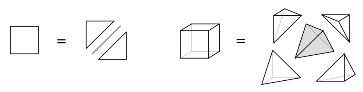
The pyramid product within the most-often used sense describes the step-up to the following dimension, using any former polytope as a base, and adding a single vertex in an orthogonal direction atop that base as a tip, thereby getting as new polytope that spanned pyramid.
For any given subdimension the subelements of that new polytope consist out of those subelements of that very dimension of the base polytope, plus the alike derived pyramids with the same tip but using any of the subelements of the base polytope with one dimension less. - This extends through all subdimension, including that of the full space on the one end ("body"), and including the empty space ("nulloid") at the other. (The nulloid, or empty set, of any polytope is unique, has dimension -1, and is incident to all subelements, including the vertices. It is the dual of the polytopal body.) The product of the empty space at the base and a single vertex (tip) being that very vertex.
The pyramid product applies especially to the dimensional set of simplices (sometimes also called: the series of pyro-polytopes). Here we get the Pascal triangle:
elemental    |                  encasing dimension D
counts       | -1     0     1     2     3      4      5      6      7       8       9      10
             |                  ({3}) (tet)  (pen)  (hix)  (hop)  (oca)   (ene)   (day)   (ux)
-------------+-------------------------------------------------------------------------------
         -1  |  1  -  1  -  1  -  1  -  1  -   1  -   1  -   1  -   1  -    1  -    1  -    1
             |     \     \     \     \     \      \      \      \      \       \       \
sub-      0  |        1  -  2  -  3  -  4  -   5  -   6  -   7  -   8  -    9  -   10  -   11
elemen-      |           \     \     \     \      \      \      \      \       \       \
tal       1  |              1  -  3  -  6  -  10  -  15  -  21  -  28  -   36  -   45  -   55
dimen-       |                 \     \     \      \      \      \      \       \       \
sion d    2  |                    1  -  4  -  10  -  20  -  35  -  56  -   84  -  120  -  165
             |                       \     \      \      \      \      \       \       \
          3  |                          1  -   5  -  15  -  35  -  70  -  126  -  210  -  330
             |                             \      \      \      \      \       \       \
          4  |                                 1  -   6  -  21  -  56  -  126  -  252  -  462
             |                                    \      \      \      \       \       \
          5  |                                        1  -   7  -  28  -   84  -  210  -  462
             |                                           \      \      \       \       \
          6  |                                               1  -   8  -   36  -  120  -  330
             |                                                  \      \       \       \
          7  |                                                      1  -    9  -   45  -  165
             |                                                         \       \       \
          8  |                                                              1  -   10  -   55
             |                                                                 \       \
          9  |                                                                      1  -   11
             |                                                                         \
         10  |                                                                              1
This small table can also be expressed as coefficients of the rational function: (1/x) · (x+1)D+1, where D is the encasing dimension and the actual power of x denotes the subelemental dimension.
The general number can be given explicitely too as: choose(D+1,d+1).
The circumradius of the simplex can be given as a function of its dimension too, just as its inradius – and thus its height, and even the dihedral angle, or its volume:
circumradius   = sqrt(D)/sqrt[2(D+1)]
inradius       = 1/sqrt[2D(D+1)]
height         = sqrt(D+1)/sqrt[2(d+1)(D-d)]     in orient. acc. to d||(D-1-d)
volume         = sqrt[(D+1)/(2D)]/D!
surface        = (D+1) sqrt[D/(2D-1)]/(D-1)!
dihedral angle = arccos(1/D)
corner angle   = arcsinD(sqrt[1/(D+1) (1+1/D)D])
(Esp. for D → ∞ we get for the regular simplex circumradius = (0||(D-1))-height = 1/sqrt(2), inradius = volume = corner angle = 0, and dihedral angle = 90°.)
Beyond this narrower sense we also could build a pyramid product of any 2 non-degenerate polytopes. Then this product will position either factor in an orthogonal subspace, but shift those subspaces relative to one-another, along a direction mutually orthogonal to both. Then all will be subject to a convex hull – at least as long both factors are convex themselves. Accordingly the dimension of this product will be the sum of the dimensions of the factors, plus one. For non-convex factors those bases could be morphed similarily, by dimensional degression, running over the set of lacing facets, which surely are pyramid products of one dimension less.
The neutral element of that product clearly is the nulloid. The pyramid product in the narrower sense is just the restriction here-of to one factor being a mere point. Further, in case both factors are uniform simplices, and the shift is adjusted so that the lacing edges also have unit lengths, this product results in (higher dimensional) uniform simplices again.
The general notation here is ×1,1, i.e. it shall consider both, the (unique) nulloid and the (unique) bulk. Let P and Q be DP- resp. DQ-dimensional polytopes, represented by their respective sets of (sub)elements P = {nd,i Pd,i : d dimension ∈ [-1,DP], i type ∈ Id}, where the coefficients nd,i represent the absolute counts (according to the diagonal elements of the corresponding incidence matrix) and Pd,i represent all types of (sub)elemental polytopes; and Q similar. Then this operator can be defined in its bivalent form by the segmentopal atop notation as:
P ×1,1 Q =
= {nd,i Pd,i : d dimension ∈ [-1,DP], i type ∈ Id} ×1,1 {me,j Qe,j : e dimension ∈ [-1,DQ], j type ∈ Je}
= {nd,i · me,j (Pd,i || perp Qe,j) : d ∈ [-1,DP], e ∈ [-1,DQ], i ∈ Id, j ∈ Je}
= P || perp Q

e.g.
triangle ×1,1 line =
= {1 nulloid, 3 vertices, 3 lines, 1 triangle} ×1,1 {1 nulloid, 2 vertices, 1 line}
= {1 (nulloid || perp nulloid), 3 (vertex || perp nulloid), 3 (line || perp nulloid), 1 (triangle || perp nulloid),
   2 (nulloid || perp vertex), 6 (vertex || perp vertex), 6 (line || perp vertex), 2 (triangle || perp vertex),
   1 (nulloid || perp line), 3 (vertex || perp line), 3 (line || perp line), 1 (triangle || perp line)}
= {(1+0+0) nulloid, (3+2+0) vertices, (3+6+1) lines, (1+6+3) triangles, (0+2+3) tet, (0+0+1) pen}
= pen
Note that the perp part in the atop notation here is quite relevant, as without that the atop notation e.g. iterates in its multivalent form into an axial stack like a tower only, while the pyramid product clearly becomes a true associative product, where any pairing contributes like in general simplices.
It shall be noted here also, that the pyramid product of a polytope P with itself, i.e. the P disphenoid = P ×1,1 P works out to be all unit-edged, provided P itself is such and the circumradius of P will be smaller than 1/sqrt(2), as then the offness height indeed would become positive. So within 3D we clearly just get tet, but in 5D we get quite generally the (n/d, m/b)-disphenoid = {n/d} ×1,1 {m/b}, or the more symmetrical n/d-disphenoid = {n/d} ×1,1 {n/d} with identical factors (the latter products then even happen to become noble and scaliform and then bow to the restriction n < 4d < 2n, if lacing edges are required to be unity too). Further, in every odd dimension the respective simplex always will be found here again. Within 7D we might think eg. of sissiddow, the gissid disphenoid, or quithdow ...
Beyond its specific application to polytope theory this pyramid product also is known within topology under the name of join.
A bit more general than the simplices obtained from the pyramid product of the former section are the simplicial polytopes, i.e. all those polytopes, which have simplices for facets only. In fact, the here obtained convex polytopes are being enlisted on the page on deltahedra (which there includes their higher dimensional counterparts too). As then the types of faces of each dimension will be unique (at least by shape – not so by around-symmetry in general), the according numbers can be non-umbiguously be given as fk for -1 ≤ k ≤ d (with f-1 = fd = 1).
For those simplicial polytopes then the set of Dehn-Summervill equations can be stated, i.e. for -1 ≤ k ≤ d-2 the following equations do hold:
d-1 Σ
j=k |
(-1)j |
(
|
j+1 k+1 |
)
|
fj = (-1)d-1 fk |
More explicitly for simplicial polyhedra there holds the following set of equations:
-f-1 + f0 -  f1 +  f2  =  f-1
       f0 - 2f1 + 3f2  =  f0
            -f1 + 3f2  =  f1
                   f2  =  f2
respectively for simplicial polychora one has the following set of equations:
-f-1 + f0 -  f1 +  f2 -  f3  =  -f-1
       f0 - 2f1 + 3f2 - 4f3  =  -f0
            -f1 + 3f2 - 6f3  =  -f1
                   f2 - 4f3  =  -f2
                        -f3  =  -f3
or for simplicial polytera one gets the following set of equations:
-f-1 + f0 -  f1 +  f2 -  f3 +   f4  =  f-1
       f0 - 2f1 + 3f2 - 4f3 +  5f4  =  f0
            -f1 + 3f2 - 6f3 + 10f4  =  f1
                   f2 - 4f3 + 10f4  =  f2
                        -f3 +  5f4  =  f3
                                f4  =  f4
and so on.
The prism product essentially is that product elsewhere in geometry described as cartesian cross-product. If both components have encasing dimensions larger than one, the result will be the duoprism thus derived. If just one component is a mere edge (1 dimensional), the product will build up the orthogonal prism atop the other component (base), and if both are 1 dimensional we get the square. Clearly, the 0 dimensional polytopal element (i.e. a point) is the neutral element of this product. Further we could consider the product of n factors, accordingly this would lead to a multiprism (triprism, quadprism, etc.).
If we just consider the step-up by 1 dimension, i.e. the second factor being a mere orthogonal edge, a similar dimensional increasing table can be derived: The subdimensional elements of any order are either those of the 2 opposite bases (doubling that number), or the prisms atop those subelements of the bases, which have 1 dimension less (adding that count). - This applies for all subdimensions of the bases, including the body, but excluding the nulloid!
The prism product applies especially to the dimensional set of hypercubes (sometimes also called: the series of geo-polytopes):
elemental   |                   encasing dimension D
counts      |  0     1     2      3      4      5       6       7        8        9        10
            |            ({4}) (cube)  (tes) (pent)   (ax)   (hept)   (octo)   (enne)   (deker)
------------+--------------------------------------------------------------------------------
sub-      0 |  1  =  2  =  4  =   8  =  16  =  32  =   64  =  128  =   256  =   512  =   1024
elemen-     |     \     \     \      \      \      \       \       \        \        \
tal       1 |        1  =  4  =  12  =  32  =  80  =  192  =  448  =  1024  =  2304  =   5120
dimen-      |           \     \      \      \      \       \       \        \        \
sion d    2 |              1  =   6  =  24  =  80  =  240  =  672  =  1792  =  4608  =  11520
            |                 \      \      \      \       \       \        \        \
          3 |                     1  =   8  =  40  =  160  =  560  =  1792  =  5376  =  15360
            |                        \      \      \       \       \        \        \
          4 |                            1  =  10  =   60  =  280  =  1120  =  4032  =  13440
            |                               \      \       \       \        \        \
          5 |                                   1  =   12  =   84  =   448  =  2016  =   8064
            |                                      \       \       \        \        \
          6 |                                           1  =   14  =   112  =   672  =   3360
            |                                              \       \        \        \
          7 |                                                   1  =    16  =   144  =    960
            |                                                      \        \        \
          8 |                                                            1  =    18  =    180
            |                                                               \        \
          9 |                                                                     1  =     20
            |                                                                        \
         10 |                                                                               1
This small table can also be expressed as coefficients of the polynomial: (x+2)D, where D is the encasing dimension and the actual power of x denotes the subelemental dimension.
The general number can be given explicitely too as: 2D-d choose(D,d).
The circumradius of the hypercube can be given as a function of its dimension too, just as its inradius, and even the angle α between adjacent facet normals, or its volume:
circumradius   = sqrt(D)/2
inradius       = 1/2
volume         = 1
surface        = 2D
dihedral angle = 90°
corner angle   = arcsinD(1)
(Esp. for D → ∞ both the circumradius and the surface become ∞ too.)
The general notation here is ×0,1, i.e. it shall not consider the (unique) nulloid, but still the (unique) bulk. Let P and Q be once more DP- resp. DQ-dimensional polytopes, represented by their respective sets of (sub)elements P = {nd,i Pd,i : d dimension ∈ [-1,DP], i type ∈ Id}, where the coefficients nd,i represent the absolute counts (according to the diagonal elements of the corresponding incidence matrix) and Pd,i represent all types of (sub)elemental polytopes; and Q similar. Then this bivalent operator is defined by:
P ×0,1 Q =
= {nd,i Pd,i : d dimension ∈ [-1,DP], i type ∈ Id} ×0,1 {me,j Qe,j : e dimension ∈ [-1,DQ], j type ∈ Je}
= {1 nulloid} ∪
  {nd,i me,j (Pd,i × Qe,j) : d ∈ [0,DP], e ∈ [0,DQ], i ∈ Id, j ∈ Je}

e.g.
triangle ×0,1 pentagon =
= {1 nulloid, 3 vertices, 3 lines, 1 triangle} ×0,1 {1 nulloid, 5 vertices, 5 lines, 1 pentagon}
= [1 nulloid} ∪
  {15 (vertex × vertex), 15 (line × vertex), 5 (triangle × vertex),
   15 (vertex × line), 15 (line × line), 5 (triangle × line),
   3 (vertex × pentagon), 3 (line × pentagon), 1 (triangle × pentagon)}
= {1 nulloid, (15+0+0) vertices, (15+15+0) lines, (5+0+0) triangles, (0+15+0) squares, (0+0+3) pentagons, (0+5+0) trip, (0+0+3) pip, (0+0+1) trapedip}
= trapedip
In other words: The prism product of P and Q is the polytope whose k-elements are prism products of the d-elements of P and the e-elements of Q, with d+e=k.
Wrt. the circumradius one here generally has the theorem of Pythagoras, for sure: r2(P ×0,1 Q) = r2(P) + r2(Q).
The volume formula is likewise direct here: Vol(P ×0,1 Q) = Vol(P) Vol(Q).
Tegum derives from latin and is ment in the sense of a coating skin of a tent. In fact, as long only convex shapes as factors are considered, the tegum product positions those within orthogonal (non-afine) subspaces, and covers the whole by its convex hull. Accordingly the dimension of the product is just the sum of the dimensions of the factors.
Esp., if one factor is just 1 dimensional, the tegum product becomes the dipyramid with equatorial cross-section being the other factor. In that case the subdimensional counts derive either from those of the cross-section of the corresponding dimension, or from those of the 2 pyramid products based each on the subdimensional elements of the cross-section of one dimension less. Considering just the counts, here those 2 pyramid products and a tegum product of that very base with an edge, would get the same numbers. This can be used for a similar dimensional iteration as for the other cases. – Again that rule applies for all subdimensional elements, here including the nulloid (which is the neutral element of the product here), but excluding the body (as the cross-section itself is not a facet of the dipyramid).
The tegum product applies especially to the dimensional set of orthoplexes (a.k.a. cross-polytopes – others call it the series of aero-polytopes):
elemental    |                  encasing dimension D
counts       |  0     1     2      3      4      5       6       7        8        9        10
             |    (q-edge)({4})  (oct)  (hex)  (tac)   (gee)   (zee)    (ek)     (vee)     (ka)
-------------+--------------------------------------------------------------------------------
         -1  |  1  -  1  -  1  -   1  -   1  -   1  -    1  -    1  -     1  -     1  -      1
             |     \\    \\    \\     \\     \\     \\      \\      \\       \\       \\
sub-      0  |        2  -  4  -   6  -   8  -  10  -   12  -   14  -    16  -    18  -     20
elemen-      |           \\    \\     \\     \\     \\      \\      \\       \\       \\
tal       1  |              4  -  12  -  24  -  40  -   60  -   84  -   112  -   144  -    180
dimen-       |                 \\     \\     \\     \\      \\      \\       \\       \\
sion d    2  |                     8  -  32  -  80  -  160  -  280  -   448  -   672  -    960
             |                        \\     \\     \\      \\      \\       \\       \\
          3  |                           16  -  80  -  240  -  560  -  1120  -  2016  -   3360
             |                               \\     \\      \\      \\       \\       \\
          4  |                                  32  -  192  -  672  -  1792  -  4032  -   8064
             |                                      \\      \\      \\       \\       \\
          5  |                                          64  -  448  -  1792  -  5376  -  13440
             |                                              \\      \\       \\       \\
          6  |                                                 128  -  1024  -  4608  -  15360
             |                                                      \\       \\       \\
          7  |                                                          256  -  2304  -  11520
             |                                                               \\       \\
          8  |                                                                   512  -   5120
             |                                                                        \\
          9  |                                                                            1024
This small table can also be expressed as coefficients of the rational function: (1/x) · (2x+1)D, where D is the encasing dimension and the actual power of x denotes the subelemental dimension.
The general number can be given explicitely too as: 2d+1 choose(D,d+1).
The circumradius of the orthoplexes can be given as a function of its dimension too, just as its inradius, and even the angle α between adjacent facet normals, or its volume:
circumradius   = sqrt(1/2)
inradius       = sqrt(1/2D)
volume         = sqrt[2D]/D!
surface        = 2 sqrt[2D-1 D]/(D-1)!
dihedral angle = arccos(2/D - 1)
corner angle   = 2D-1 arcsinD[1/sqrt(D)]
(Esp. for D → ∞ we get inradius = volume = 0 and dihedral angle = 180�, which shows that the ∞-dimensional orthoplex becomes a flat honeycomb, in fact one with a finite circumradius!)
As a nice coincidence consider the general formula: cos(2a) = 2 cos2(a) - 1. Applying that to the dihedral angle of the regular simplex provides: cos(2 arccos(1/D)) = 2 cos2(arccos(1/D)) - 1 = 2/(D2) - 1. I.e. the dihedral angle of the D2 dimensional orthoplex equates to twice the angle of the D dimensional simplex!
The general notation here is ×1,0, i.e. it shall consider the (unique) nulloid, but not the (unique) bulk. Let P and Q be once more DP- resp. DQ-dimensional polytopes, represented by their respective sets of (sub)elements P = {nd,i Pd,i : d dimension ∈ [-1,DP], i type ∈ Id}, where the coefficients nd,i represent the absolute counts (according to the diagonal elements of the corresponding incidence matrix) and Pd,i represent all types of (sub)elemental polytopes; and Q similar. Then this bivalent operator (restricted to convex figures) can be defined using the hull and the orthogonal sum operator (A ⊕ B = (A,0) ∪ (0,B)) by:
P ×1,0 Q =
= {nd,i Pd,i : d dimension ∈ [-1,DP], i type ∈ Id} ×1,0 {me,j Qe,j : e dimension ∈ [-1,DQ], j type ∈ Je}
= {nd,i me,j hull(Pd,i ⊕ Qe,j) : d ∈ [-1,DP-1], e ∈ [-1,DQ-1], i ∈ Id, j ∈ Je}
  ∪ {1 hull(P ⊕ Q)}

e.g.
triangle ×1,0 pentagon =
= {1 nulloid, 3 vertices, 3 lines, 1 triangle} ×1,0 {1 nulloid, 5 vertices, 5 lines, 1 pentagon}
= {1 hull(nulloid ⊕ nulloid), 3 hull(vertex ⊕ nulloid), 3 hull(line ⊕ nulloid),
   5 hull(nulloid ⊕ vertex), 15 hull(vertex ⊕ vertex), 15 hull(line ⊕ vertex),
   5 hull(nulloid ⊕ line), 15 hull(vertex ⊕ line), 15 hull(line ⊕ line)}
  ∪ {1 hull(triangle ⊕ pentagon)}
= {(1+0+0) nulloid, (3+5+0) vertices, (3+0+5) S-edges, (0+15+0) L-edges, (0+15+15) SLL-triangles, (0+0+15) So2oS&#L} ∪ {1 hull(triangle ⊕ pentagon)}
= hull(triangle ⊕ pentagon)
(Short edges (S) of the provided example are those of the defining unit-edged triangle resp. pentagon. Long edges then are of size sqrt(r{3}2+r{5}2) = sqrt[(25+3 sqrt(5))/30] = 1.056940, connecting the respective vertices of the defining perpendicular polygons.)
In general the tegum product is dual to the prism product. Just as prism products with both factors being larger than 1-dimensional is being called a duoprism, such a tegum product likewise is called a duotegum. But as the Catalans generally are not unit-edged, and as can be seen from the afore mentioned example, esp. the length of the lacing edges highly depends on the shape of the defining factors. E.g. when one factor is a q-edge and the other is a unit-sized orthoplex, then the product becomes the unit-sized orthoplex in the next dimension, i.e. it happens to be all unit-edged again, as the above table shows. Despite the non-unit sized q-edge (which is nothing but the exceptional 1D member of unit orthoplexes) one even gets the more general result, that the tegum product of a d-dimensional unit orthoplex and a D-dimensional unit orthoplex happens to be nothing but the (d+D)-dimensional unit orthoplex. In fact the lacing edge size will be quite generally sqrt(r12+r22) where rk are the circumradii of the factors. – Hence there are other such all unit-edged examples, resulting from unit-edged factors, eg.
The convex ones thereof then obviously provide CRF polytopes of accordingly summed up dimensional space. Moreover the tegum products with both factors being identical and at least scaliform polytopes, obeying again that (combined) circumradius property (which thus resolves to rk = 1/sqrt(2) here), would clearly result in an at least scaliform outcome in turn. Similarily a corresponding tegum product of n identical factors, again with rk = 1/sqrt(2) each, would serve here alike. In fact, this simply is because each pairwise lacing edges should become unity and thence all individual circumradii in the case of n > 2 are forced to be the same. However, orbiform polytopes still would be obtained more generally from not all identical orbiform factors with rk = 1/sqrt(2) each.
Beyond its specific application to polytope theory this tegum product also is known within linear algebra under the name of direct sum. But here in fact it is more than just a sum of the orthogonal components, as it incorporates specifically all these elements of the hull of that compound, while those 2 spanning sections thereof themselves only become internal pseudo facets. This might be the reason why this tegum product also is been found under the name free sum instead.
A volume formula can be provided as well, even so it isn't as direct as for the prism product. But because those two products are each others dual, i.e because of dual(P ×1,0 Q) = dual(P) ×0,1 dual(Q) one can obtain the the following formula here:
(dim(P ×1,0 Q))! Vol(P ×1,0 Q) = (dim(P))! Vol(P) (dim(Q))! Vol(Q)
Having mentioned the tegum product, being the hull of the fully orthogonal sum, i.e. A ×1,0 B = hull( A ⊕ B ) = hull((A,0) ∪ (0,B)), we get a close relation to the mere tegum sum (by some authors also refered to as "thatching"), which is defined by A ◊ B = hull( A + B ) = hull( A ∪ B ). Within the extended Dynkin symbol notations this tegum sum translates into that of degenerate zero-height lace prisms with pseudo bases:
extended-dyn(P ◊ Q)  =  (( 2-layer-dyn(P, Q) ))&#zx

e.g.
extended-dyn( x,w-rectangle ◊ w,x-rectangle )  =  ((xw2wx))&#zx     ( = x4x, octagon)
extended-dyn( q-tet ◊ dual q-tet )             =  ((qo3oo3oq))&#zx  ( = x4o3o, cube)
For sure, the tegum sum of 2 fully orthogonally placed components again results in the tegum product of those components.
Note that this A ∪ B itself will be nothing but the compound of A and B. Thus the tegum sum of the addends (or "layers") alternatively could be called the hull of the compound of the components.
While for the tegum product the bodies of the factors did not contribute, as was already given by the second index of the above being used multiplication symbol, but also becomes evident from the hull of their orthogonal span. Within the tegum sum, where the resulting dimension clearly is the maximum dimension of that of the factors, their bodies obviously do not contribute either for true facets. That is, "Galoomba" 's dotted regions notion, as when applied to extensions of Coxeter-Dynkin diagrams, where from its surrounded part never all nodes contribute at the same time, would apply here too: the full bodies of the factors, as being represented by the individual layers of this symbol, are to be neglected. This is what in here could be marked additionally by this region boundary - or within typewriter-friendly inline notation with the above given enclusion by ((...)).
Historical note: tegum sums had been brought up in 2014 as a further polytopal operation by W. Gevaert and this author. Dotted regions were brought up in 2022 by "Galoomba" as a concept specifically for hyperbolics with non-simplicial domains. From end of 2025 on the author adopted that concept, deviced an according typewriter-friendly inline notation and subsequently used it in this site whenever such facet restrictions do occur.
If by antiprism of some polytope P indeed is meant, as was implied by the being refered page, to be nothing but a lace prism which has for bases P and the dual of P, then one gets a noteworthy formula, which relates these antiprisms with two of the afore mentioned products. In fact one has the following result:
antiprism(P ×1,1 Q) = antiprism(P) ×1,0 antiprism(Q)
(Sure, the same holds for multiple factors each.)
For instance consider the following primary illustrating example: let P = line and Q = {3}. Then antiprism( line ) = square and antiprism( {3} ) = oct. Thus the right side of the equation would be square ×1,0 oct = tac. On the other hand we have line ×1,1 {3} = pen. So the left side indeed provides antiprism( pen ) = tac as well.
Note that the above provided reworded definition of antiprisms (in contrast to the refered to usage) is only applicable in an abstract polytopal sense, as long as the height of that antiprism would not be defined somehow as well. And indeed the above formula was derived in this very setup. On the other hand one should be aware that the absolute displacement of the pyramid product as such likewise is not defined in a more general view, when it only is to be taken as "somewhere" above. And finally remind also the mentioning at the tegum product about the sizes of its lacing edges: those were restricting by the law of Pythagoras applied to the circumradii of their factors. Thence this formula after all more comes out to relate these various free heights by a further restiriction, that very equation. But conversely, when the overall shape happens to be all unit edged, then not only the lacing edges of the left equation side's antiprism are forced to be unity, but also the edges of its bases as well. Therefore the lacing edges of the pyramid product too are bound to be unity, and the starting polytopes as well. Still, the lacing edges of the right side's antiprisms would be fixed in size thereby, but not both be bound to unity even in that setting.
A further class of 4D applications even could be seen directly for P = point and Q = {n} from the following lace city:
o-n-o   o-n-x


  x-n-o   o-n-o
i.e. the antiprism of n-pyramids (as top to bottom lace prism) = bipyramid of n-antiprism (as upper left to lower right lace tower), which is nothing but the family of n-apt (n-antiprism tegum). Note that in here the size of the (implicite) line segment connecting those two apices of the bipyramid, i.e. the P-antiprism of the formula, is a function of n even for otherwise all unit edges. In fact this n-apt would be inscribable into a circumsphere only for n=3 and that mentioned line size then clearly becomes q.
This last example then also makes the proof of the formula quite visual:
(P,0)    (0,Q)


  (0,Q*)   (P*,0)
in fact, the top is just the P-Q-pyramid, the bottom is its dual, thus that lace prism is the antiprism thereof; on the other hand the main-diagonal is the P-antiprism, the secondary diagonal is the Q-antiprism, both diagonals are to be taken orthogonal, thence these define the overall shape, the tegum product thereof. And, for sure, this shown 2D lace city representation of position space could moreover be extended to a multidimensional lace hypercity for products with even more factors, as then those polytopes P, Q, R, ... would be situated at the vertices of some according dimensional orthoplex where pairs of duals are situated in antipodal positions. And indeed, the top (or bottom) layer then becomes a simplex of position space, representing exactly that required pyramid product.
This product again is a cartesian cross-product or direct sum. Therefore nulloids do not contribute in the sequential hierarchy. But because tilings and honeycombs are infinite polytopes without body, that one is to be omitted here as well. Further, as total counts are infinite (and within this infinitude even with an exponent according to the filled dimension), only relative frequences make sense. In fact, vertex counts are to be multiplied (the =- or \\-marked "additions" really should be represented by N-tuple lines here, and N → ∞); this results in prefactors for vertex counts (resp. the relative frequences) which all equal 1.
The honeycomb product applies especially to the dimensional set of hypercubical honeycombs.
elemental    |                   filled dimension D
counts       |  0      1        2        3        4         5         6         7         8          9         10
(N → ∞)      |       (aze)   (squat)  (chon)   (test)    (penth)    (axh)  (hepth)
-------------+--------------------------------------------------------------------------------------------------
          0  |  N0  =  N1  =    N2  =    N3  =    N4  =     N5  =     N6  =     N7  =     N8  =      N9  =      N10
             |      \\     \\       \\       \\       \\        \\        \\        \\        \\         \\
sub-      1  |         N1  =  2.N2  =  3.N3  =  4.N4  =   5.N5  =   6.N6  =   7.N7  =   8.N8  =    9.N9  =   10.N10
elemen-      |             \\       \\       \\       \\        \\        \\        \\        \\         \\
tal       2  |                  N2  =  3.N3  =  6.N4  =  10.N5  =  15.N6  =  21.N7  =  28.N8  =   36.N9  =   45.N10
dimen-       |                      \\       \\       \\        \\        \\        \\        \\         \\
sion d    3  |                           N3  =  4.N4  =  10.N5  =  20.N6  =  35.N7  =  56.N8  =   84.N9  =  120.N10
             |                               \\       \\        \\        \\        \\        \\         \\
          4  |                                    N4  =   5.N5  =  15.N6  =  35.N7  =  70.N8  =  126.N9  =  210.N10
             |                                        \\        \\        \\        \\        \\         \\
          5  |                                              N5  =   6.N6  =  21.N7  =  56.N8  =  126.N9  =  252.N10
             |                                                  \\        \\        \\        \\         \\
          6  |                                                        N6  =   7.N7  =  28.N8  =   84.N9  =  210.N10
             |                                                            \\        \\        \\         \\
          7  |                                                                  N7  =   8.N8  =   36.N9  =  120.N10
             |                                                                      \\        \\         \\
          8  |                                                                            N8  =    9.N9  =   45.N10
             |                                                                                \\         \\
          9  |                                                                                       N9  =   10.N10
             |                                                                                           \\
         10  |                                                                                                  N10
This small table can also be expressed as coefficients of the polynomial: [N · (x+1)]D, where D is the filled dimension and the actual power of x denotes the subelemental dimension.
The relative coefficient of the general number can be given explicitely too as: choose(D,d).
The general notation here is ×0,0, i.e. it shall neither consider the (unique) nulloid, nor the (unique) bulk. (Note that within this context we speak of infinite polytopes, not of tesselations. When considering tesselations, the not to be used bulk surely is omitted already.) Let P and Q be once more DP- resp. DQ-dimensional polytopes, represented by their respective sets of (sub)elements P = {nd,i Pd,i : d dimension ∈ [-1,DP], i type ∈ Id}, where the coefficients nd,i represent the absolute counts (according to the diagonal elements of the corresponding incidence matrix) and Pd,i represent all types of (sub)elemental polytopes; and Q similar. Then this bivalent operator can be defined by:
P ×0,0 Q =
= {nd,i Pd,i : d dimension ∈ [-1,DP], i type ∈ Id} ×0,0 {me,j Qe,j : e dimension ∈ [-1,DQ], j type ∈ Je}
= [1 nulloid} ∪
  {nd,i me,j (Pd,i × Qe,j) : d ∈ [0,DP-1], e ∈ [0,DQ-1], i ∈ Id, j ∈ Je}
  ∪ {1 (P × Q)}

e.g.
trat ×0,0 aze =
= lim N → ∞ {1 nulloid, N vertices, 3N edges, 2N triangles, 1 bulk} ×0,0 lim M → ∞ {1 nulloid, M vertices, M lines, 1 bulk}
= {1 nulloid} ∪
  lim N,M → ∞
  {NM (vertex × vertex), NM (vertex × line),
  3NM (line × vertex), 3NM (line × line),
  2NM (triangle × vertex), 2NM (triangle × line)}
  ∪ {1 (trat × aze}
= lim K → ∞ {1 nulloid, (K+0+0) vertices, (K+3K+0) lines, (0+3K+0) squares, (0+0+2K) triangles, (0+0+2K) trips, 1 bulk}
= tiph
The neutral element for this product here would ask for something consisting out of 1 nulloid, 1 point, and 1 edge. In fact it is the monotelon, i.e. the tiling of the projectively closed 1D space ("line") with a single point ("vertex") on it.
Despite its original application to infinite euclidean structures, in fact it simply focusses on the surface only. And as such it well becomes applicable to finite structures as well, such as their (finite) maps on torical spaces, or other (infinite or finite) skew tilings.
However, just as the prism product ×0,1 surely is to be considered the default product for finite polytopes, so likewise the comb product ×0,0 is to be considered the default product for infinite "polytopes".
As a historic remark it shall be noted that Mrs. Krieger originally denoted the comb product exactly in the same way as the prism product, i.e. concatenating the factor Coxeter-Dynkin diagrams without any product sign as a reducible symbol, then applying just the implicite guide, that products of finite factors are to be taken as prism products, while products of infinite factors are to be taken as comb products. In 2022 however "Galoomba" then introduced as visual guide into according graphical diagrams his "dotted lines", thereby enclosing diagrammal regions, which do not allow for all of their nodes to be taken (cf. to "×.,0"). Those graphical devices got introduced into the typewriter friendly inline notations only at the end of 2025 by using double parantheses ((...)) around the according factor symbols. I.e. CD(P ×0,0 Q) = (( CD(P) )) (( CD(Q) )).
The general demicubes clearly are not defined by a product, they not even are regular. Rather they are defined secondary by an alternation of the hypercubes. But it might be interesting here to derive some general, only dimension dependent formulae for this infinite polytopal series as well. To that end simply consider the following picture, providing the general idea within dimension 2 and 3 each:
Obviously from a unit hypercube a total of 2D/2 = 2D-1 corner simplices, each of hypervolume 1/D!, are to be subtracted. The remainder then is a rescaling, in fact the transition from the cubical edge as a unit to that of the demicube. That one is a linear scaling by sqrt(2), but, because the volume surely would be D-dimensional (for D>2), it therefore results in
volume = (1 - 2D-1/D!) / sqrt(2D)
(For D=2 that formula a posteriori would become valid too, but only within a measure theoretic sense: the diagonal edge clearly is subdimensional wrt. an area measuring, and thence the formula given value of 0 here indeed applies also.)
This section serves as a short intro to the |,>,O devices (provided independently by P. Pugeau and Quickfur), its relations to the affore mentioned products, and then esppecially will be devoted to explicit applications.
These devices contain 3 symbols. Each represents a specific building operation, all increasing the dimension by 1. They all start with a mere 1D element, the edge, being displayed by |. (In fact, one might start with a point . instead. But then, the action of any of the symbols, being apllied to it, would result in a line segment. Therefore that part can be omitted, and the number of symbols directly corresponds to the dimension of the resulting figure.)
The first such operation is the extrusion ("|"). It is nothing but the afore mentioned prism product.
It uses some object as base, and extrudes that object up to the opposite base, therby nowhere changing that cross-section. This operation is
likewise represented by | (sometimes also alternatively by the more typewriter-ready capital letter "I"),
being attached at the right to the so far compiled |,>,O device for the base.
Especially || therefore describes the square.
–
Algebraically the application of ..| could be described by abs(... - an xn) + abs(... + an xn) = a0.
The second operation is the tapering (">") of some base with one opponent point.
It thus describes the afore mentioned pyramid product.
Its symbol is a > sign (sometimes also alternatively by the more typewriter-ready capital letter "A"),
attached to the right of the so far compiled |,>,O device for the base.
The simplest example here is |>, describing the triangle.
–
Algebraically the application of ..> could be described by abs(... - an xn) + abs(...) = a0.
Finally this symbolic set also includes a spin ("O") advice, producing all sorts of round things.
The action of that operation will be denoted by a trailing O symbol.
(Note, that this is the point where Quickfurs notion would differ. He originally just intended some round bi-tapering, which led to lots
of crude shapes. The spin operation of Pugeau here definitely serves better, providing plenty of highly interesting shapes.)
–
Algebraically the application of the latter ..O could be described by sqrt((...)2 + an2 xn2) = a0.
But as we here are related to polytopes, we restrict here to few examples only:
Whereas the spin operation in effect seems to commute with either one of the formers, extrusion and tapering definitely do not. – In the followings we will omit any applications of the spin. Restricted thus, then any iterated application of both, of extrusion and of tapering, clearly remains within the set of segmentotopes only. This is because each such application just adds a single additional vertex layer within a further, perpendicular dimension.
As usual, we then will consider unit edges only. Surely this does not provide any restriction to the extrusions. But for the taperings this amounts for the starting figure (corresponding to the very symbol, but without that last > sign) that those should have an circumradius which is lower than unity: else lacing edges of unit size cannot connect the base vertices to the tip anymore! (Note that the circumradius itself here clearly does exist, as we are dealing with segmentotopes.)
| 1D | 2D | 3D | 4D | 5D | 6D | 7D |
|---|---|---|---|---|---|---|
| - edge |
|| - {4} |> - {3} |
||| - cube ||> - squippy |>| - trip |>> - tet |
|||| - tes (R = 1) |||> - cubpy (R = 1) ||>| - squippyp ||>> - squasc |>|| - tisdip |>|> - trippy |>>| - tepe |>>> - pen |
||||| - pent (R > 1) ||||> - tespy (H = 0) |||>| - cubpyp (R > 1) |||>> - cubasc (H = 0) ||>|| - squasquippy (R = 1) ||>|> - squippyippy (R = 1) ||>>| - squascop ||>>> - squete |>||| - tracube (R > 1) |>||> - tisdippy (R > 1) |>|>| - trippyp |>|>> - trippasc |>>|| - squatet |>>|> - tepepy |>>>| - penp |>>>> - hix |
|||||| - ax (R > 1) |||||> - (pentpy) † ||||>| - (tespyp) ° (R > 1) ||||>> - (tesasc) ‡ |||>|| - squacubpy (R > 1) |||>|> - (cubpyippy) † |||>>| - (cubascop) ° (R > 1) |||>>> - (cubete) ‡ ||>||| - cusquippy (R > 1) ||>||> - squasquippypy (H = 0) ||>|>| - squippyippyp (R > 1) ||>|>> - squippypasc (H = 0) ||>>|| - squisquasc (R = 1) ||>>|> - squascoppy ||>>>| - squetep ||>>>> - squepe |>|||| - tratess (R > 1) |>|||> - (tracubpy) † |>||>| - tisdippyp (R > 1) |>||>> - (tisdipasc) † |>|>|| - squatrippy (R > 1) |>|>|> - trippyippy |>|>>| - tripascop |>|>>> - trippete |>>||| - tetcube (R > 1) |>>||> - squatetpy |>>|>| - tepepyp |>>|>> - tepasc |>>>|| - squapen |>>>|> - penppy |>>>>| - hixip |>>>>> - hop |
||||||| - hept (R > 1) ||||||> - † |||||>| - † |||||>> - † ||||>|| - ° (R > 1) ||||>|> - † ||||>>| - ‡ ||||>>> - ‡ |||>||| - cube cubpy (R > 1) |||>||> - † |||>|>| - † |||>|>> - † |||>>|| - ° (R > 1) |||>>|> - † |||>>>| - ‡ |||>>>> - ‡ ||>|||| - tes squippy (R > 1) ||>|||> - † ||>||>| - ° ||>||>> - ‡ ||>|>|| - squa squippyippy (R > 1) ||>|>|> - † ||>|>>| - ° ||>|>>> - ‡ ||>>||| - cube squasc (R > 1) ||>>||> - squisquascpy (H = 0) ||>>|>| - squascop pyp ||>>|>> - squascopasc ||>>>|| - squasquete ||>>>|> - squeteppy ||>>>>| - squepep ||>>>>> - squix |>||||| - trapent (R > 1) |>||||> - † |>|||>| - † |>|||>> - † |>||>|| - squatisdippy (R > 1) |>||>|> - † |>||>>| - † |>||>>> - † |>|>||| - cubtrippy (R > 1) |>|>||> - † |>|>|>| - trippyippyp |>|>|>> - trippypasc |>|>>|| - squatrippasc |>|>>|> - tripascoppy |>|>>>| - trippetep |>|>>>> - trippepe |>>|||| - tettes (R > 1) |>>|||> - † |>>||>| - squatetpyp |>>||>> - squatetasc |>>|>|| - squatepepy |>>|>|> - tepep yipppy |>>|>>| - tepascop |>>|>>> - tepete |>>>||| - cubpen |>>>||> - squapenpy |>>>|>| - penpyp |>>>|>> - penpasc |>>>>|| - squahix |>>>>|> - hixippy |>>>>>| - hopip |>>>>>> - oca |
So far we considered the subset obtained by extrusion and tapering. – However there is a somehow related set of convex polytopes, then obtained from extrusion and bi-tapering ("♢"). Those polytopes then are fully described by any sequence of application of the prism product and the tegum product, again being applied to a starting edge line. Alternatively these well could be defined equivalently by an according sequence of the prism product and the dualisation operations instead. In fact this class is also known as that of the Hanner polytopes.
It should be noted that in general unit-edged bipyramids come out either as tall or as flat, i.e. dull in any case! Moreover those polytopes are neither segmentotopes nor all unit-edged lace towers generally any longer. However there is a different normalization possible for all Hanner polytopes: Coordinates could be taken to be chosen from {+1, 0, -1} instead.
Up to this renormalization (i.e. requiring still all unit edges none the less) we would get the following list. However some here would
become impossible then (cf. †).
* Within the mentioned rescaled sense of Hanner polytopes this becomes a square again and so ||... and |♢... would
be the same generally. While in the here prefered all unit-edged sense it rather would have been a 60° rhomb instead.
However then we will run into non-regular faces and, when further bi-tapering, into different edge sizes directly for any of the |♢... .
Thence those subsequent ones in the listings below got omitted.
| 1D | 2D | 3D | 4D | 5D |
|---|---|---|---|---|
| - edge |
|| - {4} |♢ - 60° rhomb * |
||| - cube ||♢ - oct |
|||| - tes (R = 1) |||♢ - cute ||♢| - ope ||♢♢ - hex |
||||| - pent (R > 1) ||||♢ - (tessit) † |||♢| - cutep |||♢♢ - (squacubdit) † ||♢|| - squoct (R = 1) ||♢|♢ - opet (H = 0) ||♢♢| - hexip ||♢♢♢ - tac |
Volume and hypervolume in here is taken to be the same. Esp. within 2D the usual area could be addressed as a volume as well when taken within the according subspace.
Volumes of such convex polytopes, which have some specific center point, could easily been calculated directly, simply by addition of the volumes of the respective pyramids, which have their tip each at the given center point and their base being any of the polytope's facets. One then observes that the choice of that center point does not really matter, i.e. any shift would increase the value of some of those facet based pyramids, while for others it declines, so that within their sum the volume value clearly remains unchanged.
Using this invariance it becomes possible to extend the volume calculation even to arbitrary orientable star-shaped polytopes as well. Here orientability is used in the sense of the (piecewise connected) manifold of its boundary surface, and star-shaped clearly is taken in the "radially convex" sense for point sets, i.e. there exists some internal point such that for any second internal point the whole line segment between those two fully remains within the inner region as well. In fact, we first divide the set of facets into prograde ones and retrograde ones. Then one calculates the volumes of all these individual facet pyramids. Finally we add all pyramid volumes for the prograde bases and subtract therefrom all pyramid volumes for the retrograde bases.
It should be noted that this very definition of volume is highly correlated to the applied "filling method". In fact it possibly dissects the internal region into such subregions, which belong to a single or any other number of facet pyramids. Again these numbers of overlaps depend on the provided facet set only and are independent of the chosen center (as long as the star-shapedness allows for more than just a single such "center"). This it true, as the lacing facets of the pyramids are false dissections where this number of overlays does not change. The respective highest number occuring throughout the total inner region of the polytope then is being addressed to as the density of that polytope. Convex polytopes clearly have density 1 throughout – if their facets are to be taken prograde.
Starryness clearly can occur on every level. Not only the polytope itself might have intersecting facets (like a gad), but also the facets themselves could be such in turn (as for sissid). As the nD pyramid volume V = h·G/n requires the volume G of its base as one of its contributing factors, the above density consideration applies on iterated levels as well. This is what sometimes got named endoanalysis. In fact wrt. any level the density consideration of this very level applies hierarchically in a bottom up way, i.e. across the facet at an internal point of its own regions the density of the respective around space changes by the amount of its own (subdimensional local) density. Thus, because for the pentagram the pointy tips have density 1, while the central region have density 2, it follows that for sissid the regions underneath the pointy tips likewise have density 1 (difference at the margin being 1), while the central region has density 3 (difference at the margin being 2). Thence that (total maximal) density of sissid is said to be 3. And accordingly the above volume definition by means of facet based pyramids indeed would count that central region three times as well. Still (in general), due to possible retrogradeness of facets, the inner subregions might get (local) densities of zero or, even worse, of negative numbers.
Specific formulae for the prism product ×0,1 and the tegum product ×1,0 had been provided already above, but will be repeated here again as well:
Vol(P ×0,1 Q) = Vol(P) Vol(Q)
(dim(P ×1,0 Q))! Vol(P ×1,0 Q) = (dim(P))! Vol(P) (dim(Q))! Vol(Q)
When considering the volume formulae provided above, it often might serve not only interesting when having the absolute values, but likewise those providing the ratios with respect to the corresponding circum- and insphere.
Speaking of sphere or hypersphere within this context, we mean not its surface, but rather the union with its bulk underneath, sometimes also called the hyperball. I.e. in 2D we won't speak of the circle, but rather of the disk. – Further, as the volume of the D-sphere scales according to D-th power of its radius, we reserve the term "unit sphere" for those with unit radius (not diameter!).
The problem in here is that the volume of the to be used D-sphere cannot be given in a closed form, except when recruiting to the non-intuitive Gamma function. So we have either to distinguish between even and odd dimensions, or we could refuge to general comparisions of dimensions D+2 with D.
volume of unit D-sphere    = πD/2 / Γ(D/2 + 1)

volume of unit 2D-sphere   = πD / [Πk=1D k]   = πD / D!
volume of unit 2D+1-sphere = πD / [Πk=1D+1 (k - 1/2)]   = 2 D!(4π)D / (2D+1)!

volume ratio of unit D-sphere with unit (D-2)-sphere = 2π / D

starting values for recursion (and few further values):
volume of unit 0-sphere    = 1
volume of unit 1-sphere    = 2
volume of unit 2-sphere    = π           = 3.141593
volume of unit 3-sphere    = 4 π / 3     = 4.188790
volume of unit 4-sphere    = π2 / 2      = 4.934802
volume of unit 5-sphere    = 8 π2 / 15   = 5.263789
volume of unit 6-sphere    = π3 / 6      = 5.167713
volume of unit 7-sphere    = 16 π3 / 105 = 4.724766
volume of unit 8-sphere    = π4 / 24     = 4.058712
...
volume of unit ∞-sphere    = 0
(That last value already shows the reason for that section: we are measuring volumes in general by hypercubical units. And we will see, that the higher the dimension, the more relative volumina will be centered at the vertex surroundings of the hypercube! I.e. the volume outside its insphere, compared to the insphere volume, gets arbitrarily large.)
For simplices we get for every even dimension that the ratio of the simplex volume Vsimplex to the volume of the respective insphere Vinsphere evaluates to
Vsimplex(D) : Vinsphere(D) = sqrt[(D+1)/(2D)]/D! : ( πD/D! · 1/sqrt[2D(D+1)]D ) = sqrt(D+1)[sqrt(D(D+1))/π]D, if D = 2n
For D → ∞ this value increases without bound. That is, the simplex eventually will have nearly all its volume outside of its insphere!
For orthoplexes we get for every even dimension that the ratio of the orthoplex volume Vorthoplex to the volume of the respective insphere Vinsphere evaluates to
Vorthoplex(D) : Vinsphere(D) = sqrt(2D)/D! : ( πD/D! · 1/sqrt(2D)D ) = [2sqrt(D)/π]D, if D = 2n
For D → ∞ this value increases without bound, but to a lesser degree. That is, the orthoplex still eventually will have nearly all its volume outside of its insphere!
For hypercubes we get for every even dimension that the ratio of the hypercube volume Vhypercube to the volume of the respective insphere Vinsphere evaluates to
Vhypercube(D) : Vinsphere(D) = 1 : ( πD/D! · 1/2D ) = (2/π)D D!, if D = 2n
For D → ∞ this value again increases without bound (in fact being for every allowed D just within the bounds of the corresponding values of simplex resp. orthoplex). That is, also the hypercube eventually will have nearly all its volume outside of its insphere!
When comparing various polytopes one might ask which one is more like a hypersphere than the other. Above we already gave a first answer to that by the comparison of the volume of the polytope to the volume of its insphere. This serves well for regular polytopes. But in general there will be no common insphere. One might want to dualize that very setup, comparing the volume of the circumsphere to the volume of the polytope. But again this might serve for orbiform polytopes only. Thus we have to dive a bit deeper for an even more general concept.
Such a general objective measure of roundness can be provided by the ratio of its body volume to its surface volume. But this sort of measure still depends on the absolute size because body volume and surface volume do scale differently wrt. their absolute size variable. For that reason let us consider the following absolute roundness measure
abs.roundness(P) = (VP)dim(∂P) / (V∂P)dim(P)
where VP is the volume of some polytope P, ∂P is its (hyper-)surface, and dim(P) is its (local) dimension. Esp. dim(∂P) = dim(P)-1 for sure. By the use of these exponents this measure now becomes scale independent. It is also known as the isoperimetric ratio.
If we further denote by abs.roundness(O) the absolute roundness of the (filled hyper-)sphere itself, then one sees a further disadventage of this so far defined measure (cf. the according explicitly provided values below): the absolute roundness is good for comparing polytopes of the same dimension, but for comparing shapes of various dimensions, e.g. of the different hyperspheres themselves, the according values vary highly with their dimensions. – This is why we further introduce the relative roundness measure as the ratio
rel.roundness(P) = abs.roundness(P) / abs.roundness(O)
Thus, just by definition, one gets rel.roundness(O) = 1 for the hyperspheres O of all dimensions. Therefore the dimensional sequences of according values for classes of polytopes P now become comparable as well.
The volume of the D-sphere, VO, was already given above. The surface contents of the D-sphere, V∂O, can be derived via differentiation wrt. to its radius R therefrom as
V∂O(R) = dVO(R) / dR

surface of unit D-sphere    = D πD/2 / Γ(D/2 + 1)   = D · volume of unit D-sphere

surface of unit 2D-sphere   = 2 πD / (D-1)!
surface of unit 2D+1-sphere = 2 D!(4π)D / (2D)!
Thus for the here relevant values of abs.roundness(O) one gets therefrom the following general formula for even resp. odd dimensions. Additionally some values for the lower dimensions are provided explicitly.
abs.roundness( 2D-sphere )   = D! / (πD (2D)2D)
abs.roundness( 2D+1-sphere ) = (2D)! / (πD (2D+1)2D 22D+1 D!)

abs.roundness( 1-sphere )    = 1 / 2             = 0.5
abs.roundness( 2-sphere )    = 1 / (22 π)        = 0.079577
abs.roundness( 3-sphere )    = 1 / (22 32 π)     = 0.0088419
abs.roundness( 4-sphere )    = 1 / (27 π2)       = 0.00079157
abs.roundness( 5-sphere )    = 3 / (23 54 π2)    = 0.000060793
abs.roundness( 6-sphere )    = 1 / (25 35 π3)    = 0.0000041476
abs.roundness( 7-sphere )    = 3·5 / (24 76 π3)  = 0.00000025700
abs.roundness( 8-sphere )    = 3 / (221 π4)      = 0.000000014686
...
Having done those calculations for the hypersphere, we turn to the series of simplices now. Their volumes and surface contents were already given above.
abs.roundness( D-simplex ) = D! / sqrt[D3D(D+1)D+1]

abs.roundness( line ) = 1 / 2                     = 0.5
abs.roundness( {3} )  = sqrt(3) / (22 32)         = 0.048113
abs.roundness( tet )  = sqrt(3) / (23 34)         = 0.0026729
abs.roundness( pen )  = 3 sqrt(5) / (29 53)       = 0.00010482
abs.roundness( hix )  = sqrt(5) / (32 57)         = 0.0000031802
abs.roundness( hop )  = 5 sqrt(7) / (25 37 74 )   = 0.000000078728
abs.roundness( oca )  = 32 5 sqrt(7) / (28 710)   = 0.0000000016464
abs.roundness( ene )  = 5·7 / (229 37)            = 0.000000000029809
...

rel.roundness( 2D-simplex )   = (2D)! πD / (D! sqrt[(2D)2D(2D+1)2D+1])
rel.roundness( 2D+1-simplex ) = D! (2π)D / ((D+1)D+1 sqrt[(2D+1)2D+1])

rel.roundness( line ) = 1                        = 100 %
rel.roundness( {3} )  = π sqrt(3) / 32           =  60.459979 %
rel.roundness( tet )  = π sqrt(3) / (2 32)       =  30.229989 %
rel.roundness( pen )  = 3 π2 sqrt(5) / (22 53)   =  13.241464 %
rel.roundness( hix )  = 23 π2 sqrt(5) / (33 53)  =   5.231196 %
rel.roundness( hop )  = 5 π3 sqrt(7) / (32 74)   =   1.898165 %
rel.roundness( oca )  = 3 π3 sqrt(7) / (24 74)   =   0.640631 %
rel.roundness( ene )  = 5·7 π4 / (28 38)         =   0.202982 %
...
Next we consider the hypercubes. Again the volumes and surface contents are given above. (Because of being measure polytopes, those here happen to be rather trivial for sure.)
abs.roundness( D-hypercube ) = 1 / (2D)D

abs.roundness( line ) = 1 / 2         = 0.5
abs.roundness( {4} )  = 1 / 24        = 0.0625
abs.roundness( cube ) = 1 / (23 33)   = 0.0046296
abs.roundness( tes )  = 1 / 212       = 0.00024414
abs.roundness( pent ) = 1 / (25 55)   = 0.00001
abs.roundness( ax )   = 1 / (212 36)  = 0.00000033490
abs.roundness( hept ) = 1 / (27 77)   = 0.0000000094865
abs.roundness( octo ) = 1 / 232       = 0.00000000023283
...

rel.roundness( 2D-hypercube )   = (π/4)D / D!
rel.roundness( 2D+1-hypercube ) = πD D! / (2D+1)!

rel.roundness( line ) = 1                 = 100 %
rel.roundness( {4} )  = π / 22            =  78.539816 %
rel.roundness( cube ) = π / (2·3)         =  52.359878 %
rel.roundness( tes )  = π2 / 25           =  30.842514 %
rel.roundness( pent ) = π2 / (22 3·5)     =  16.449341 %
rel.roundness( ax )   = π3 / (27 3)       =   8.074551 %
rel.roundness( hept ) = π3 / (23 3·5·7)   =   3.691223 %
rel.roundness( octo ) = π4 / (211 3)      =   1.585434 %
...
Then there is the series of orthoplexes (aka cross-polytopes). Their volumes and surface contents are provided above as well.
abs.roundness( D-orthoplex ) = D! / (2D sqrt(D3D))

abs.roundness( line ) = 1 / 2                    = 0.5
abs.roundness( {4} )  = 1 / 24                   = 0.0625
abs.roundness( oct )  = sqrt(3) / (22 34)        = 0.0053458
abs.roundness( hex )  = 3 / 213                  = 0.00036621
abs.roundness( tac )  = 3 sqrt(5) / (22 57)      = 0.000021466
abs.roundness( gee )  = 5 / (211 37)             = 0.0000011163
abs.roundness( zee )  = 32 5 sqrt(7) / (23 710)  = 0.000000052686
abs.roundness( ek )   = 32 5·7 / 237             = 0.0000000022919
...

rel.roundness( 2D-orthoplex )   = πD (2D)! / (23D DD D!)
rel.roundness( 2D+1-orthoplex ) = πD D! / sqrt[(2D+1)2D+1]

rel.roundness( line ) = 1                     = 100 %
rel.roundness( {4} )  = π / 22                =  78.539816 %
rel.roundness( oct )  = π sqrt(3) / 32        =  60.459979 %
rel.roundness( hex )  = 3 π2 / 26             =  46.263771 %
rel.roundness( tac )  = 2 π2 sqrt(5) / 53     =  35.310570 %
rel.roundness( gee )  = 5 π3 / (26 32)        =  26.915171 %
rel.roundness( zee )  = 2·3 π3 sqrt(7) / 74   =  20.500183 %
rel.roundness( ek )   = 3·5·7 π4 / 216        =  15.606620 %
...
If the hypervolume of a parallelotope is P and the subdimensional hypervolumes of its n facet parallelotopes at a specific vertex v0 are Pk for 1 ≤ k ≤ n then the hypersine of the hypersolid corner angle of that specific parallelotope vertex v0 can be defined (in conformance with the 2D case of planar geometry) as
sinn(v0) = P/(∏0≤k≤n Pk)
Using this definition then it follows by restriction first to according simplices, and then by using the polar sine wrt. the simplex facet opposite to v0, that the hypersine of v0 can be related to the dihedral angles αjk between the simplex facets Sk, which are incident to v0, by
              |     1      -cos(α12)  ...  -cos(α1n) |
(sinn)2(v0) = | -cos(α21)      1      ...  -cos(α2n) |
              |    ...        ...     ...     ...    |
              | -cos(αn1)  -cos(αn2)  ...      1     |
A direct application to any of the hypercubes provides αjk = π/2 for all 1 ≤ j,k ≤ n, i.e. sinn(v0,hypercube) = 1 here generally (again in conformance with the 2D case of planar geometry).
A different application to any of the regular simplices provides αjk = arccos(1/n) for all 1 ≤ j,k ≤ n, i.e. the hypersine here generally evaluates to
(sinn)2(v0,simplex) = (n+1)n-1 / nn = 1/(n+1) (1+1/n)n
As the latter factor here converges to the Euler number e, the hypersine of the hypersolid corner angle of the regular simplex clearly would converge to zero.
In order to calculate the hypersine of the hypersolid angle of any orthoplex, we would have to divide the hypersolid angle into simplicial portions first. Just consider x3o3o...o3o4o (orthoplex) as being the vertex figure of x4o3o3o...o3o4o (hypercubical honeycomb). That is, each looked for subsimplex is nothing but the vertex corner pyramid of an hypercube – just that the vertex of consideration, i.e. which contributes to the vertex corner of the orthoplex, would be one of its base vertices. Thus the contributing subsimplex corner angle could be derived as
                         |      1          0     ...       0      -1/sqrt(n) |
                         |      0          1     ...       0      -1/sqrt(n) |
(sinn)2(v0,subsimplex) = |     ...        ...    ...      ...         ...    | = 1/n
                         |      0          0     ...       1      -1/sqrt(n) |
                         | -1/sqrt(n) -1/sqrt(n) ...  -1/sqrt(n)       1     |
And therefrom we clearly get at least
v0,orthoplex = 2n-1 v0,subsimplex = 2n-1 (arcsinn)[1/sqrt(n)]
(Note the attached index n to both the sine and the inverse sine functions in order to remind that we are dealing with hypersine instead of usual 2D sine only.)
© 2004-2026 | top of page |
