©  ©

©

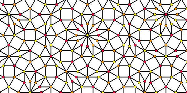
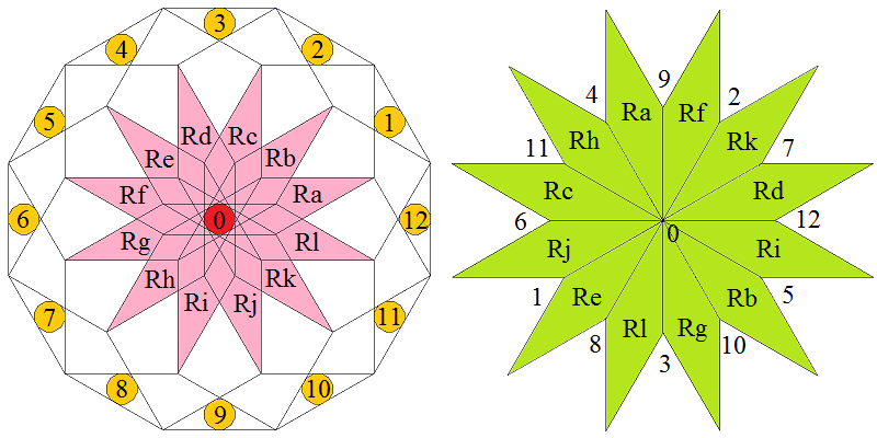
The right picture above provides a consistent 3-coloring of the rhombs and squares, as found in this article. For that purpose first the vertices would have to be colored in such a way, that any edge always carries 2 different (out of 3) colors on its ends. This rule already induces the coloring around any triangle by all 3 colors each, and for the remaining vertex type 12 the coloring is induced as complement of the 2 colors of the 12 neighbouring vertices. Wrt. the rhombs and squares in addition it is required that always 2 colors are used at a single corner each, while the remaining 2, within opposite positions, carry the third color. So far these vertex coloring rules still cannot be applied too far, as the freedom at the tetragons would stop its further application. Even so in this tiling it is quite often, that a vertex is surrounded by a complete dodecagon of one but next neighbours. As can be spotted in the left picture, it happens that the central color is also applied at this dodecagon at every alternating position (inscribed hexagon), whereas the other 2 colors then will alternate in the remaining spots (inscribed triangles). The high frequency and the overlaps of these dodecagons finally allows for a local application of this 3-coloring of the vertices. – In order to get a coloring of the tetragonal tiles, as depicted above, simply the majority color of their vertices is used in a second step.

Vertex configurations & acceptance regions

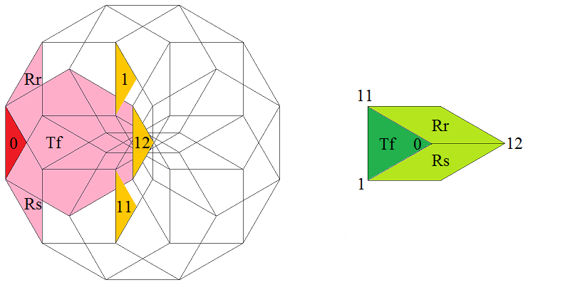
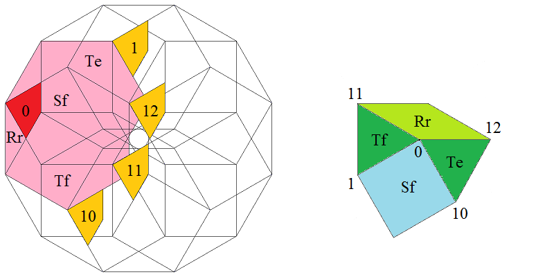
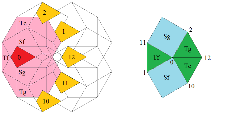
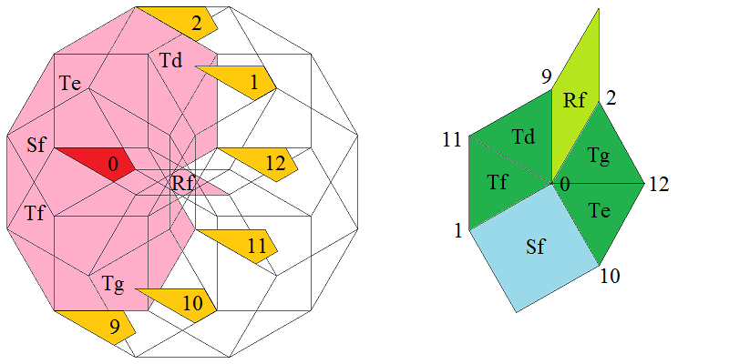
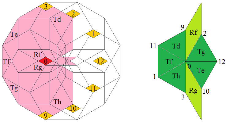
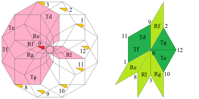
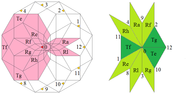
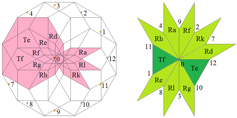
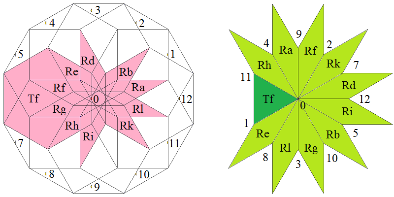
At the left the dodecagonal acceptance domain, which corresponds to the projection of a single Voronoi cell, which here is a hiddip into the perp space. At the right the corresponding vertex configurations of the tiling space are shown. There the incident tiles are projections of the polygonal faces of the Delone cell, which here is a triddip. Accordingly the tiles all are either triangles or tetragons, the latter of which within the chosen projection either squares or (30°,150°)-rhombs, whereas the triangles remain regular. Within the following table the different regions of the acceptance domain are marked in red (and additionally labeled as "0"), which 1 by 1 correspond to the shown vertex configuration each.

When lifting the incident tiles of tiling space back into embedding space, and selecting the dual Voronoi cell boundary of that specific Delone cell boundary, the corresponding projection shadow into perp space always is shown there in rose. These acceptance domains of tiles also are labeled accordingly by "S_" (for squares), "R_" (for rhombs), resp. "T_" (for hexagons and triangles). Obviously the red regions are just the common intersections each of those rosaic tile domains. Btw., the prism products of alike marked regions of tiling space (tiles) and of perp space (their acceptance domains) happens to be the corresponding Klotz. (This is why the hexagonal regions of the domains in perp space and the triangular tiles both have been labeled "T_": they are nothing but the shadows of the same Klötze.)

Finally the relative edge shifts likewise are lifted back into perp space (shown in yellow and labeled with mere numbers). Therefrom then the exact incident next vertex configuration could be deduced, provided that the exact relative perp space coordinate of the starting "0" vertex is given. Here only true edges have been lifted; the likewise one edge length detached vertices between two neighbouring rhombs could be spotted within the acceptance domain as further, here not shown region shifts. – In fact, these tilings all happen to belong to a single local isomorphism class, the specific representant can be coded by that starting perp space coordinate c_⊥. Thereby then the full infinite tiling is defined completely.

Type 1 relative frequency = [2 sqrt(3)-3]/36 = 1.289171 % count of orientations = 12	Type 2 relative frequency = [9-5 sqrt(3)]/18 = 1.887478 % count of orientations = 12
Type 3 relative frequency = [14 sqrt(3)-24]/9 = 2.763459 % count of orientations = 12	Type 4 relative frequency = [33-19 sqrt(3)]/6 = 1.517244 % count of orientations = 12
Type 5 relative frequency = [26 sqrt(3)-45]/6 = 0.555350 % count of orientations = 12	Type 6 relative frequency = [123-71 sqrt(3)]/12 = 0.203272 % count of orientations = 12
Type 7 relative frequency = [97 sqrt(3)-168]/18 = 0.049602 % count of orientations = 12	Type 8 relative frequency = [459-265 sqrt(3)]/36 = 0.018156 % count of orientations = 12
Type 9 relative frequency = [362 sqrt(3)-627]/36 = 0.006645 % count of orientations = 12	Type 10 relative frequency = 97-56 sqrt(3) = 0.515478 % count of orientations = 1